Terrain Terracing Algorithm

Reposting this in a different format. Basically considers not fully implemented ideas concerning edge contour curve construction, and delves into the matter of how one might terrace model a terrain mesh object.

I have considered the following solution as a thought out non implemented exercise to a problem which not only involves terrain edge detection but edge detection at a given height, hence defining a surface edge contour curve.  

   

   The problem defined here is as the title states a terracing problem.  One can visualize this with real world examples found throughout the world, in particular in the use of land space as in the case of agriculture, say rice plantations on a given mountain side, or sweet potato plantations.  Here we descriptively define the use of such space as increasing a given elevation surface area of land space by cutting into a given hill/mountain side until having reached a terrace’s defined spatial surface area allotment.  Then commencing the process of terracing the procedure is repeated on subsequent higher elevation layers until having reached a maximum height of such hill/mountain side.  

   Some alternate descriptive ways of characterizing a terrace as follows:

• A terrace can be also defined as a land surface contour where the contour of the terrace represents some closed loop of a given surface region.  
• The surface area of contour loop may be thought of as in the layered cake analogy of a particular region that is extruded to some height level, and that a neighboring terrace is a contour loop that is either nested and extruded or contains the nested extrusion of any subsequent contour regions.  

Defining the Contours of the Map

Consider the mathematical descriptions and possible requirements involved in defining a contour of a terrace:

1. Cataloging all known height positions.
2. Checking for contiguity between positions...this means checking to see if the contour is closed loop passing through any similar height map position, or having defined a contour loop in its own right.
3. Linearly interpolating between points (an edge), to determine where a non identified vertex need be created potentially in further identifying a contour.

Once having defined the contours of the map, one can imagine a top down topographical approach here.  That is, a two dimensional map has defined curvature that shouldn’t be like a hiker’s map in so far as defining elevation curvature of a given landscape.  A similar construction could be applicable in the aid of the terracing problem likewise.

For a given contour, for points that are not defined on the grid (conforming to, for instance, a defined grid subdivision), one could define this more clearly to the minimum spatial resolution (if desiring equal spacing between all grid points), or having used an approximation such as choosing a nearest neighbor assignment in further defining the contour.  

If we restricted our terracing problem in way that we are restricting the maximum number of potential terraces, then the problem is potentially likely a destructive or constructive process, depending on the number of potential identifiable conto urs present.  

For the destructive or constructive case, likely we’d want to, according to scale, consider the maximum number of contours distributed in some fashion across the scale of such terrain.  That is, we’d work upon the principle of best matching a terrain terrace height elevation to identified height map regions on the grid.  In this case defining matching and neighbor proximate vertices within these terrace elevation regions.  

Thus likely the problem could be defined in a number of variational ways here.

  Nearest neighbor vertex solution  

Let’s say we have the following

Obviously in the figure we can see a two dimensional representation of a top down contour shows how many potential nodes are missed for a given grid of a provided resolution.

One solution to this problem is to choose nearest neighbor points representing the contour.

         

Here we can see this is an approximation to the contour line.  By choosing the nearest neighboring point we can ensure that the contour is more closely represented to a fixed dimensional grid size...where vertex position points, for instance, are spaced metrically in equal ways from one point position to the next.  The trade off on this with lower resolution is that there may be more significant loss in graphic data representing the curve.

Since mesh objects can be represented, however, in various ways, we need not alway represent say a contour line by way of equally spaced points either in representing such mesh object.  Meaning we can also choose to structure an object with vertices as we choose.  In this way we can also re represent a curve conforming to a new set of points

Changing the resolution of the grid

  While the nearest grid point choice method, allows, still allows a contour to be better represented in terms of data on a given fixed resolution grid.  One might also consider changing the resolution of the grid.  This amounts to increase the amount of potential vertex data for a given terrain mesh object.  Thus coupling this with a nearest neighbor vertex method, one might reduce loss/change in geometric data, but also add potentially increasing the size of such data by increasing the resolution of the object (that is, by increasing the number of vertices representing a given terrain objects form).  

 

Re representing the curve

In the next sequence we merely re define the set of mesh points using an algorithm which structures the set of mesh points according to a defined curvature.  We can actually define such curvature, for instance, using a cubic spline approximation along the loop, and thus defining equal point spacing on a given contour by using something like arc length formulation piecewise for each spline equation.  While this defines probably a better approximation for a given mesh contour along the terrace, however, this does present problems for defining the mesh object further in so far as say faces and/or determining the application of texture objects.   Secondly we for a given mesh object whose vertex spatial arrangement is given according to a uniquely defined contour surface based coordinate system, we still contend with the issue of determining inside such curve the coordinates of points.  We could use something like surface based normals alongside a scaling procedure which determines the next set of interior points, repeating this procedurally as necessary until having reached an adequate contour welding surface to any neighboring contour.  Admittedly this is also a much more complex mathematical prospect, although one should imagine if having been completed successful could provide for arguably the least geometric loss in data.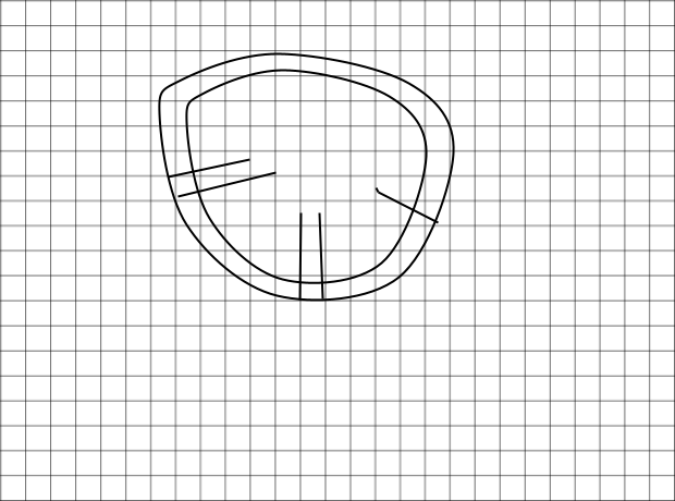  

Procedurally not only would one need contend with drawing the contours at any given heightmap level, but again determining based upon the set of edge normals provided from each edge welding faces from one contour band to the next.  Higher resolution data, not doubt likely reduces potentially the difficulties encountered in such problem, although something like a normal lines from neighboring points intercept problem could be key in solving this sort of problem…

The diagram to the left illustrates for instance, roughly drawn normals relative to contour lines.  Ideally the same number of points are drawn even as the scaling of the contour line diminishes, which is to say that as the contours become smaller and smaller in terms of arc length the number of vertices remain the same.  Thus the faces diminish in surface area size as the contour arc length becomes smaller.  

There are some problems, however in the distribution of points per contour surface area.  Consider the sawtooth ridge problem.  Here if a given ridge line were drawn as one contiguous closed loop boundary, we’d likely have the same problem as a continuously drawn set of contours, that ideally under rescaling reached an apex where total points distribution were one and the same.  However, in the non contiguous sawtooth ridge problem, we instead subdivide the ridge line into several closed loops and at some point must distribute between these closed loops a total number of points in keeping to the original contiguous closed loop problem.  That is the spatial distribution of points might like similar except subdivided between closed loops at a given apex.   Obviously we’d need to account for repetition of points along such boundary curvature like wise as illustrated below…

 

Here the dotted line in the figure might represent for a given spatial area a contiguous ridge line (which aids in the formation of a solution) since this dotted line approximates what a total distribution of points would look like, we could then approximate a distribution of points for each peak.  In this case a distribution, for instance, might be given according to a matching of spatial area as related to the contiguous case.

This particular problem also may be best approached in a different way entirely.  Which is that one might instead define a contour say from a base level, and then attempt to path construct an edge normal which should intercept adequately a neighboring contour normal.  This ostensibly turns into something of a path finding problem with optimizations since one need to join two normal edges ideally so that as close to a linear approximation is yielded in the process of finding an normal edge relative to either defined neighboring  contour curve.  

If between two contours a non adequate path is found, perhaps, an intermediate contour might be constructed which parses differences between both such curves so as to situate a path as close to being a linear normal edge as possible?!  In any event, one might also resort to constructing normal curves within tolerances ranges for path construction.  Once an adequate normals path resolving method is found.  For any arbitrarily chosen point on the contour curve, and given arc length point wise distribution (for a given curve base), one can commence building the set of normals path wise along the perimeter of a base contour, until having traversed the set of all potential points on a given circumference.    Reminding in theory we should be able to do all this as long as we have piecewise built the set of all contour curves with their corresponding families of cubic spline interpolated functions...we’d start by computing normals of such function say between cubic spline point intervals on the contour.  This leads into another potential algorithm described below.

Path wise intermediate contour construction algorithm

 The example works as follows, between two neighboring contours pathwise normals are constructed and we optimize on a given inner curve the a point normal which closely approximates as needed a linear pathwise normal curve between both such curves, but that such point still neither yields a pathwise normal say on the inner contour within a prescribed threshold range.  In this case, we can draw from either point normal linear curves and then compute an intercept point.  From this intercept point we can draw another curve that more smoothly transitions the pathwise normal curve, defining an intermediate contour.  We could fill in the details of the intermediate contour, however, a bit differently than as in the previous set of algorithms which constructed a contour set.  Instead the path wise normal determines the two dimensional coordinate positions with a defined function for such normal (in this case we are likely resorting to another interpolated function of second or third order criteria).  Secondly along such path with regularly defined contours of a given metric definition (whether this were spacing defined in regular intervals of a few meters elevation), we could resort to some regularity provided by average on such pathway.  If such spatial length were distributed at say 40 meters elevation, then the path’s mid elevation range on average would be 20 meters upon normals intercept...or however distant in scaling relative to a midpoint or the end points in determining the elevation for an intermediate contour.  One particular topographical rule is that at least contour elevation bands themselves may be set by some regularized interval (whether this were 5, 10, 15, and so forth meters).  The spatial distance from normal point to normal point on the other hand between neighboring contour curves, on the other hand, may vary so that larger scale elevation change has taken place with relatively small path wise normal distance gained.  A path wise normal curve, also, optimally represents on the family of contours, the shortest path for maximum elevation change, or in field topology, for instance, may represent the direction of say ‘force’ on a given field space….consider the example of gravitation space time topology...the normals on such field contour would represent the direction of force at at any given point on such space time continuum.    The advantages also in terms of field topology having terrain mesh topology constructed in such a way, is that these may compliment field simulations.  Consider for instance, the direction of hydraulic terrain deformation characteristics.  More easily if these normal contour paths are determined in the readied sense, computational expense may be less so if considering say the problem of probabilistic path of water transport and sediment deposition.  Of course, this does lead to an added problem of reconfiguring curve contours on a post deformation cycle.  

Constructing the contours

   This problem can be considered in a number of ways.  If it is a topographical map, that one had in hand, one would simply need scan an image while simultaneously threshold reading relevant versus non relevant data.  In this case, we’d likely have depending on the resolution of the image a bit mapped representation of the image, which means that our contours would need be interpolated pointwise in defining topographical data.  

  Another problem is reading the data say from a mesh object with a more commonly given equi distant metric provisioned on a terrain mesh object, this tends to be common for non organic mesh representations while organic structures on the other hand might have topology defined more closely in the way of topographical contouring.  In the event of contouring an object say using Cartesian based (affine) coordinate systems, you’d need to have linear interpolation methods set in determining where for instance, points on the mesh objects correspond to a given contour, or constructing contours using contiguous closed loop determining routines from limited mesh object spatial data sets.  What one should have for a given contour is not a set of points (although we could define a contour in this manner) but a family of functions say for point wise intervals (one could set this interval at something an equidistant range of 1 integer unit, although this equidistant range need not be anything as large as one integer unit)...I don’t recommend integer unit intervals ranging significantly large since cubic functions become unstable over larger numeric intervals (these will lead to pronouncements in say path oscillations which renders stability in curvature useless).    This leads to a subset of the problem at hand…

   Determining a contour cubic spline function for a given contour interval   

First in this problem for the described interval, it would be presumed one have adequately mapped a set of points.  In a rough way, one should have an algorithm which sketches out a contour (in a preprocessing manner) one might imagine.  Part of this pre processing appending/mapping of data, may look for things like nearest neighbor points for a given curve contour...this is not simply an algorithm which matches all points to a given terrain elevation, but also need sense points that may be contiguously drawn into a contour in its own right.  Consider the twin peaks problem where two peaks may share up to a point similar contour bands but are non contiguously drawn between banding regions.  Thus one should have a property which determines that a contour may be drawn from such point to a neighboring point of the same elevation...thus some search criteria means that not only a point shares the same elevation, but that edges along such path intercept the contour band.  It may help in principle also using a process of elimination when having constructed a sequence of contour points.  Discarding points in the algorithm that have already been appended to a contour region.  Ideally what one should have in the preprocessing stages are not only some definition of the contour region points, but that the spacing of points are ideally proper for spline interpolating...ideally these could be in whole integer units (and one may need some procedural method for normalizing the set of data so as to make this condition mathematically proper and ideal for interpolating).  Linear interpolation will obviously come in handy since edge making algorithms not only tell us without computing the neighbor points on such edge that an a contiguous contour may be defined, but that linear interpolating processes will tell us exactly where such edge intercepts on the contour’s two dimensional coordinate plane.   In this respect, it would be expected that the process of determining contiguity also has furnished a necessary spatial arrangement of data (given pre processing normalization).  Once such data is readied then it is merely a matter of processing such data from the cubic spline interpolated process on the the two dimensional contour plane.  In this way, the simplest algorithm it suffices would likely have some computed slope data provided (say left approach one boundary point and left approach simultaneously on another boundary point), obviously the boundary points themselves should have been computed in the preprocessing stage.  Then we’d merely append the cubic function coefficients and procedurally repeat this process working circumferential around the contour curve until having amassed for such curve the family of functions describing the curve with corresponding map provisioned between point intervals, both x and y...keep in mind we’d have two matching local x coordinate position for two separate functions so likely a two coordinate key tuple matches best the coordinate to function.  Procedurally we repeat this sequence for the set of all contours on a banding region, and then repeat this process yet again for all such delineated contours.

Some added things for consideration especially in pre processing data include:

  key indexing data for fast retrieval...consider the neighboring point problem where a known neighboring interval is being sought after for a given point.  In this case, something like the moore neighbor search problem, or von neumann problem I’d imagine suffices.  Thus pre processing neighbor point key data for a given point could readily speed up a given search for neighboring points on the search algorithm problem.  Again one isn’t merely searching to see if a neighbor point is at such a height, but that it has an edge crossing such contour boundary….even if a neighbor point is at another heightmap value greater or lower than a respective contour position this doesn’t meet sufficiency for the contour criteria, a neighboring point could be proximate at the same contour height but doesn’t have an edge that crosses the contour plane, and is technically interior to the contour curve (that is, define and defining any other contour curves but not the one that we are looking for)...such a point must have an edge that crosses the plane of the contour, or be positioned exactly on the contour itself.  Imagine the cross section of an apple, the edge defining the contour at every such horizontal cross section of the apple (xy plane).  In this way, if a point on the apple also intersecting the plane of such contour isn't defined, an edge between vertices on the apple should be crossing and cutting into the contour plane for such given cross section.  

Having this one can then proceed to the next step…

Computing the normal of a contour curve

The family of function provides this answer to us in directly via calculus, for instance, and a bit of trigonometry.  We can compute the tangent of the curve (first derivative), and then compute from this the normal using trigonometry on the tangent line (90 degrees relative the tangent).  Other methods for computing normals from a known equation may work likewise.  It is important keeping reference to direction, there are actually an infinite number of normals (rotated around the plane of a tangent curve).  We are actually looking for a normal curve that is on the contour plane, and is likely specified with direction since path wise we’d likely be moving in one direction along such normal to the set of interior contours.

Optimizing the path normal between two contour curves

 If such a problem were given to the simplicity of a rescaled contour curve, likely there would be little work needed in finding point intercept on a neighboring nested contour curve, since this position should using something as simple as point slope formulation...that is a linearly projected along the path normal intercepting the interior contour curve represents the normal also to such interior curve.  

In principle this approach could be applied likewise, and then a given test performed to see how the direction of the normal  (on the point slope intercept) compares to the point interval’s normal (from the contour’s function on such interval).  In this case if there are significant deviations between the point intercept normal and the interior contour curve normal, then one may need consider constructing a set of pathwise contours which transform the path normals to reconcile better to desired tolerances.    The idea here is subdividing say the ‘error’ between two curves neither matched at a given point for curvature.  Methods for smoothing a curve’s ‘error’ can be done also by again interpolating a normal pathwise curvature.  Where boundary condition endpoints are determined and normal’s provided by either boundary points are again provided which in turn provide first derivative conditions of the path wise normal...in this way we have all the ingredients lined up for another cubic spline interpolated normal curvature along the path normal.  Once having this we can articulate the curve by determining intermediate contour points which describe more smoothly transition from one one contour region into the next.   Technically if this subdivision were infinitum, there would be no discernible ‘error’ given between contour transitions, and the normal path would be perfectly described as perfectly normalized at the intercept of each contour curve.  

There are some caveats to a path tracing algorithm in finding a best fit from one contour curve to the next.  Optimization should include that the path is the least linear distance in summation between both points from their respective point normal curves.  This is not by the way the least distance as given by euclidean distance in a cartesian coordinate system between two contour curves.  The optimal path is determined rather by the path of normals which can be thought of as an extension of a local surface coordinate system.  It is implicitly assumed that by extension of the most optimal linear path, an optimized cubic equation will likewise result in terms of arc distance.  The optimization routine for choosing such path could use something like an iterated newton’s method...basically from a test point value if path distance appears to be growing larger, then on an iteration cycle an upper bound is constructed on the previous iteration, while refining a midpoint iteration between the upper bound its parent lower bound.   In this way we hone in closer and closer to an optimal point, in a given testing routine.  One can likely set an upper limit in ‘error’ testing between the any previous iteration successor and a likely most optimal point candidate, whether this is a very small decimal point running, for instance, in the range of .000000001 or something like this, generally this all being contingent on desired computational expense.  Likely I visualize this problem as optimizing in the linear case, and then constructing the cubic equation describing such path, otherwise, added computational expense occurs both in computation of the cubic equation and its given arc length measurement.  Obviously the linear case, is quicker and easier.

From a given base subdivision of a contour arc we can apply rule for as many points on any closed contour loop.  The first ancestral successor likely is given to an algorithm of our choosing in so far as the allocation of points subdividing the contour.   Any given generational contour successor will already uniquely through the path routine describe above have its assignment of points on the contour curve, so one only need construct, in theory, one particular arc length subdivision on the curve.  All other contour curve subdivisions will follow suit from this ancestor.  

Additional Rules for Contour Loops

  We can additionally consider the construction of some following rules for contour construction:

1. A contour that has no child successor will be given to a midpoint subdivision...this is ideally a mid point arc that that traverses the length of the contour curve.
2. Any series of contour curves in a banding region given to an absence of child successor contours will have a midpoint arc that flows between such contours forming an inter connecting bridge between such loops, or in other words, where a parent contour has more than one child successor means that midpoint arc bridge should be constructed between such child closed loops.  Consider, for instance, the saw tooth example given above. We’d construct between the peaks a sub ridge maximum arc curve subdividing this parent contour curve of the saw tooth peak contours.  

Really at the moment I can only visualize the necessary special construction rules in these two special cases.

The construction of the midpoint arc curve may be given by the following process for rule 1:

1. We’d follow a similar procedure to the normal path optimization routine, except the mid point will be constructed on special case premise.  An optimal path will be constructed from a pair of known points since both points will have been determined.
2. Once choosing an optimal point (opposite side of the contour curve), a cubic curve can be subdivided at approximately equal to ½ its total arc length…
3. Once having appended all such points on the closed loop we can construct the final midpoint ridge of the closed curve.  

The construction of midpoint arc curve for rule 2 on other hand appears to be a composite of standard rules and the rules given:

1. Where no child optimal point successor is found and that it appears that an optimal point on the parent is instead found determines the use of such parent point (opposite side of the contour curve).  

This provides more or less a description of the processes involved in contouring a terrain.  Likely given that terrain is appended in terms of surface topology that is euclidean in nature...one may need weld any of this topology to an existing framework in providing compatibility, or otherwise re translating...some game engines like ‘unity’ will not accept anything but a standard euclidean based surface topology (where the spatial surface metric between points is the same).  On the other hand a number of three dimensional modeling programs may easily accept any of these types of surface topology.  In ‘Unity’ you’d likely import these terrain structures as mesh object.

Building the terraces

  Once having a set of contours plotted two dimensional in any event allows one either by extrusion, or by some method of translating points on the contours.  Most of the work is completed at this point, and all processing of data up to this point provides relation to contour data.  In this regard, contour data contain level banding data, meaning that terrain data is given at a constant height between contour regions, and that the contours themselves represent the change in elevation relevant to any successor region that is banded at higher or lower elevation.  If creating a family of functions mapping representation of the a given surface topology, as has been the focus of much of this writing up to now, ultimately there would be a transformation of functional data into object data points, like vertices and their face correspondence.  Obviously, this leaves another algorithm which constructs both the set of vertices and their respective point positions in some global euclidean coordinate system, but also a given inter relation between the vertex indices and, for instance, their face and edge data structures.

   Probably the simplest of organizational structure of vertex container data, follows an ordering regimen that is not unlike reading the data say from the page of a book.  Whether an object topology is read from top to bottom, and running left to right, followed by the next line feed after one line is completed.  The extension of this organizational routine would be applied in so far as face data organization.  This does leave however, some potential complications when surface topology is organized a bit differently.    Thus it is probably important when reading surface vertex data, that the order reading scheme of vertex data might otherwise be the same if the surface topology were cut and rolled out as a flat piece of paper.  Another method that I could think of, in the case of contouring organizes vertex data by way of principle of the contours themselves.  Where one say chooses consistently say a twelve o’clock position and then reads clockwise or counter clockwise around the contour, a map is also constructed relating this contour to its child(-ren) successor(s), and then presumably at the same heightmap another contour is read given to some geographic ordering principle, whether this is in the fashion of reading a book from top down, left to right, until all contours at such heightmap level are read.  Once completing this cycle a next elevation heightmap band is read repeating the same algorithm.  All of this is repeated into all heightmap representations are completed and no further contour data remains.  Obviously preprocessing relational data can speed up search and mapping aids between vertex  data.  For instance, when normal paths are constructed between neighboring contours, neighboring point relations can be pre appended to relational maps that save us having to construct this data on a next go around when appending vertex relational data for constructing faces of the terrain object.   Thus in the previous steps above prior to the terrain object construction we actually should have mapped vertex data, and thus likely we should have vertex key data mapped even before we commence in defining the positions of vertices or their faces technically.  In this respect then it may also be important for preprocessing face data in so far as vertex ordering before the positions of the vertices have been assigned, and if we have done this, likely it may be a small step in mapping coordinate data as this could also be easily computed in the processing stages above.  With these maps having been constructed implementation may already be done for us if we consider the ordering of how we are processing data...its not so hard to add a few steps that save us a lot of added work later if we consider well the process of computations here.  

  Thus I recommend actually if in defining contours, using the routine of building a family of functions both of contours and normal curves on such contours, also simultaneously indexing vertex coordinate data, as well as mapping face data by vertex indices...customarily mapping face data amounts to building the face using the vertex’s index position followed by any neighboring vertices forming the face in a clockwise or counter clockwise manner.  Thus a square face could be represented as [0,1,2,3] where each integer position represents the stored vertex’s index position in the vertex coordinate data container that might look like [[0,0,0],[0,1,0],[1,0,0],[0,0,1]] is probably the most common representation of a face.  A face can have more and less than four vertices representing a face (called triangles and faces likely having poles...when they have less or more than 4 edges).

Summation:  Likely the nearest neighbor vertex solution coupled with resolution dynamics to a given surface topology, could make for easier implementation for building curve contours.  Albeit you’d still need to determine the contours using a similar method as defined above as in constructing contours that involved building a family of spline functions, that is in defining where the edge boundaries of the contour curves exist, the process should be much the same.  There appears to be some added labor involved in functional curve building (spline building case), but on the other hand allows us to specifically tailor our terrain topology as needed by vertices that we choose to represent in such geometry, such method not only optimizes potentially a better representation of terrain terraced surface topology but allows us to represent by whatever desired resolution in so far as our application is desired. (where surface spatial metrics between points are the same).  The more crude method allows us to change the resolution of the grid to more closely approximate the contour data, but may do this with some added computational and rendering expense.   I’d leave it up to the reader to see if there were any appreciable difference in so far as computational expense for either method.  Lastly, as has been pointed out with respect to the matter of organic topology if surface topology could be given the same respect in terms of structure, one could appreciate the sorts of flowing structure better represented in terms of surface terrain allowing for some furthered ease in changing terrain structures.  Often times I imagine this is an easier point to neglect since one could seldom think less of terrain animations...for instance, hills need not eyebrows that need be easily moved up and down, or have some skeletal muscle structure in a similar way that might simulate animated motions, for instance, a smile, a frown, or anything of this sort that might more amply necessitate or provide furthered use for better surface topology, on the other hand, maybe some practical use could be had of the type of well contoured surface topology that might be had relative to other approximating cases?  In any event, this could at least be eye candy for 3d terrain modelers.

Brush off the math books again...all of this entails use of linear algebra, calculus, and so forth.  Some key things to be implemented:  Computation of the cubic spline equation.  Computing derivatives, computing arc length, and trigonometry, or if you were interested in the mathematics of geography, this is an excellent applied mathematics project.

A given life philosophy question

   I am thinking about this in some considerate way, and maybe haphazard way.  Honestly, one should think considering any manner of previous condition that one should be destined in one way or another.  Whether it were supposedly a decline by the nature of one's existence, in any event, however, leading to the same circumstantial condition before.  This culmination ends likely where it started so many years ago, in the same circular recess, one should imagine, and amazingly whatever generational persistence could have pushed any similarity by that very condition.

     Existential questions one could offer shouldn't be as likely in the same ways given to the passing of decades, aging, nor something like mid life crisis, then more humorously the sort whim of another's judgement, appropriating any more air of mis judgement as to condition.  As to the concentration of values, however, such are likely given, an alien circumstance, is neither given so well to easily writing off, as it were likely in other circumstances, or more likely given that supposedly that anything might be reflexive enough in passing.  

     If a new day is like a birth which strangely as it seems it should ever be, there is also something less brooding of an existence.   A given evocation obviously to the sort of instilled judgement that one might have concerning life, and manner of value placed upon it...it seems conditionally speaking I might value at least any previous learning that I would have and has only aided and enhanced survival, in absence to basic necessities, and then admittedly something of a voice somewhere.  It seems balancing something of the attributes of life, material possession, career, and anything else worldly in nature is always limited...of course, mid life crisis I'd offer could be enhanced by some suffering to all power in mindset placed in this way, if it weren't only to the extent an absence somewhere likely to be discovered, and to be spared another going to and from any likely certain worry wrought in time to the sleepless wanderings, so much that one's inset malaise were likely to the consolation of a lengthier sleep, consideration of change might be a given.  As to the priority of one's worldly pursuit, likely it is mindful that they are limited and very much worldly it would seem more often, and certainly it would seem least likely to persist upon death.

Then passing into the years. 

Little of this in question, and it seems there must be fortune, one should imagine. 

Value then it seems is likely where one should have found something less abyssal in mind.  If it were digress, there should be an uncertainty by way of the force, given to moving.  On the other hand, any previous routine, however, thoughtless from previous work leads to any less than well observed condition.  Here this last statement, less than well observed, is more often I think likely to the ritual of a tenured existence, and why feeling rebirth must be a highly nuanced feeling at that relative to first adult child steps.  At least the feeling shouldn't be, 'not another ounce of this.'  Existence is measuring and controlling, if one could do so, the degree of suffering experienced in life...not that in the long term that one might always be the wiser.

I am not certain that there is growing more sensitive or less sensitive to any condition, that makes for one's existence.  If this should seem all the same as in the previous years, at least in the continuance of anything, unless there were some revelation had of it, and if only revelation had commenced in forming the idea of any retreat otherwise.  

Hopefully as in getting older, one is not so much the more callous, at least it seems owing to any ignorance in life passing, there is much callousness already...these sorts of exteriors can't last forever.

   

Thoughts and interpretations on the Perlin Noise Algorithm

Perlin noise

  I've examined the algorithm and could weigh in a little opinion geometrically speaking concerning the algorithm.  Mostly this is likely echoing a number of blogs on the subject matter.

  Firstly as a key to the algorithm, there are a number of key components to the method:

  A gradient field is given to random noise generation.  The gradient field itself appears to be randomly generated, but the actual coordinate position do not have randomly generated noise.   If this were the case, each and every point would be incoherent in terms of noise relations which is certainly not the case, meaning that each an every coordinate point would be entirely random and such a noise field would appear truly as something like 'white noise', instead there is an inter relation between the coordinate positions and randomly generated gradient noise.

  In the two dimensional case, the mathematics that one might describe geometrically speaking is given to a process of vector magnitude product weighting between the Gradient field at its coordinate node point (these, gradient nodes are given to whole integer coordinate representations), and the actual coordinate position which is not required to be coincident to any node but between them...in other words, the actual 2d (x,y) coordinate position is any real number coordinate representation and not restricted to the two dimensional set of integers (I,J) that the gradient field is restricted.  The actual dot product formulation geometrically is the magnitude product of two vectors in the direction of one such vector.  This can be thought of as product weighting in other words, but its not necessarily the same as mathematical averaging.

All coordinate positions in two dimensions, falls inside of a four coordinate gradient node grid position...that is on the set of integers, any real two dimensional coordinate can be found inside a integer boundary derived square.  There are plenty of blogs that mention this example by example, so I'll avoid further expounding on this.  This square however that forms the boundary of the coordinate position is where the gradient nodes (vertices of the gradient square) come into play determining the noise at such coordinate position.

Each particular gradient coordinate node is actually weighted according to the non gradient coordinate position, that is, between the gradient node and the coordinate position that we wish to compute in so far as a perlin noise value.  Once the dot product between all surrounding gradient node positions have been computed which determines each coordinate to node weighted gradient 'noise' scalar (at a given gradient node), a linear interpolation takes place between the upper and lower y node boundaries on both given x axis respectively, this determines the Perlin noise interpolated position at the actual coordinate x position between such weighted gradient scalars on the upper and lower boundaries of the gradient grid coordinate system, and then having computed the linearly interpolated position for the y coordinate position between the gradient nodes upper and lower y boundaries.    We are determining a noise factor between all such weighted node gradient scalars to the actual coordinate position.  This noise has coherence because of a drawn mathematical coherence between a randomly generated gradient noise field and the mathematical smoothness provided both in weighting the gradient field according to individual coordinates coupled with interpolating processes which graduates the degree of randomness so that neighboring coordinates are inter related in a quasi statistical like manner concerning the randomly generated gradient noise field.  Basically the coordinate position's noise comes by way of the influence of four different gradient node positions (nearest to such coordinate), and as one more closely approaches a coordinate point from a neighbor position, similarities in noise should mathematically occur in the two dimensional problem.

I'd say additionally that the gradient field seems a bit fancy, likely a good choice of descriptive words, but basically could be the same as saying a randomly generated vector field in another way.  Unless I am missing something by way of the mathematics here.  Generating the gradient field in two dimensions is given to the restriction of a random vector bound to the unit circle, for example, or not really a complicated process.   

Windows installation experience

   After several re installations of Windows, coupled with being an install tester with Linux, I can give some personal summary as to the difference between Windows and Linux in so far as which is likely more light weight and quicker with the install, and which is likely to contain unnecessary bloat ware.

    Hands down, if you were knowledgeable on this subject matter, you'd likely guess right on the issue of Windows being the slower of installation, likely the more cumbersome, and supposedly if you thought it were likely more free of being error prone, in my experience, as of today, really not so true.  Especially consider when security updates generating errors on an install means sitting for hours (and these are literal hours) waiting for restore points to be re enacted.  For the amount of time spent waiting around, one could have windows re installed to exactly a given restore point several times over!  Amazing that re store points take so long!

   As to Linux, not that security is necessarily any better, but at least if you are screwed on the issue of security you hadn't need be pre occupied with the computer for hours on end waiting to push the OK button for one security update relative the other.

Typical windows re installation time:  several hours minimum when the installation works, this includes waiting around for security updates or any system updates.  Much of the time spent waiting is preparing, it would seem the desktop/laptop for updates (as in pre process scanning and deciding which apparent packages were necessary), coupled by an even lengthier process.

Typical time for a linux OS installation:  20 to 30 minutes usually.  And maybe another 20 to 30 minutes for package updates....I am not sure if .ISO installers tend to be more current in terms of implemented packages, kernel updates, and/or anything which makes the state of the Operating likely more current relative to the often given commercial ISO on the windows side that tend to be floating out there.  While Linux may not out of the box handshake in every possible way with big brother adobe flash (for playing more commonly any videos on YouTube, Amazon Prime streaming, Netflix,or anything like this)...technically Linux mint and Ubuntu variations I believe do up to a point and the usual work around for completely enabling streaming for Amazon prime or I'd imagine Netflix is done (at least for me). 

Possible Theory?

Reason all this might matter?  Well for most maybe it matters little, I'd suspect most people don't like to touch their computers.  And likely why if you were into servicing windows at least from the standpoint of re installing it, such interface is more cumbersome, slow and generally undesirable.  On the other hand, the typical linux user learning curve maybe a tad bit more than the average windows user, and then coupling this with software groups actually interested in attracting prospective customers.  The quicker, the simpler, the easier it is to get an operating system installed added with any number of points to user experience is likely to resonate with some potential base not only in initially installing but persistently using an operating system.  Likely there are plenty of web posts that layout where operating system users dominate, on the other hand, and its generally one product in so far as world wide markets...that's Windows, and not much else.  Linux on the other hand accounts for supposedly a share of approximately one percent.  While Windows accounts for a bulk majority of users out in the markets.  Although some interesting trending appears to be occurring amidst the share of users in this arena.  Any persistent number of users now appear to be using, for instance, generally no longer supported (outside of commercial vendor software) legacy Windows XP operating system, considering that this market is something like 14% of a given user share in the total market and tied with a Windows 8 user share market, while Windows 7 dominates the reset of the field.

Part of this could be because for an existing user base, interoperability issues between legacy hardware and newer operating systems tend to be more difficult, although this may not necessarily be true for alternative operating systems outside of Windows XP.   The other issue could be a given user demographic, coupled with consumer malaise in certain areas of the computing industry.  This may come down to an issue of people are likely to want to upgrade their smart phone before they put another hulking piece of machinery that stays fixed in the living room, and likely serves as another fixture to the family entertainment center.  The laptop certainly has lost fashionable attributes, and mostly any other fixture, could be described more likely as specially devoted, outside of the swiss army like utility that a smartphone device might possess, and here Windows is pretty much almost non existent in so far as the common user is concerned.

It seems if one were perusing the arguments for marketing relevance, clear and easy to read screens, coupled with faster potential silent forms of communications (given by keystrokes as opposed to voice command) could be reasons for any technological renaissance.  Mostly, however, in terms of productivity needs, in a personal way, any sort of larger scale computing device should have some obvious advantages over the smaller compact stuff out there.  If ever cloud computing software usurped this any further, likely the necessity of these more cumbersome pieces of hardware could be relegated to any vast cloud warehouse having sprung up...mainframe models to industries and the personal computer as one should know it a relic.

In the meantime, given to user relevance, I could still argue that Windows might embrace appreciably some models and methods that linux computing should offer.  Whether it were ease in installation, simple, more free of bloat ware, were quick, clean, crisp, sharp, leaving users with excellent graphical experience...and I'd say graphical experience were part of this.  While I've read some suggesting that graphics rendering should be provisioned at a stage of irking a consumer...it would seem this is the poorer approach to consumer marketing.  If it weren't more obvious that some headway were supposedly needed to computational data analytics on things like resource mining, it might seem the share of space on one's computer were devoted to other things that had little to do with a given user.  Obviously, for whatever users that have been interested in maintaining a Windows device, it would seem that marketing here has been often times poor enough, and statistics have much to show for this.
Then given the level of user experience, where it seems more commonplace that paying for intrusion should be a pretty masochistic activity in its own right, paying for poorer use of technology, or paying for lower end content suffices? 

All of this likely would better work, where any level ignorance abounded, better success would have been had, if, for instance, a government insisted that a technology remain in place as it had, maybe a telecommunications service were ensured up and running to the exclusion of any other service...thus, imprisoning individuals for broad band voip services, but much of this were like providing amply the taste of a forbidden fruit, and playing the role of a serpent all at once.  Unfortunately, knowledge of states hadn't aided in this situation, or at least if intending to lord ignorance, it seems one should do a better job at disinformation, or merely all of this suspect claim is more self evident in a government that amply picks up on opportunity at political hand grabs like a *****.
  

Amazing stuff

I can't even install Windows completely, but I can install other operating systems now on the ole laptop!

Hmm, pre and post election state, I know there must be opportunism here!

By the way Chrome installations are down on Linux mint, at least for all my computing devices.

I'd suppose there'd be some urging for Dropbox installation...kind of reminds of recent role playing where some dude is like 'man I have dropbox can we share using that... and I'm like 'I use Drive, not Dropbox...'  I ended laughing at this bit of insistence.

not that I suppose it matters a whole lot these day if you were really into security on cloud stored data.

Strange deal

I have two identical versions of the same laptop.  One laptop was responding right away with an F2 entry into bios at the initialization state screen.  While the other one weren't, so I went to investigate about the last known bios virus which were something like 1999, pretty rare deal although supposedly I've read of possibilities of these sorts of infections aiding in the mbr resets, or basically when one goes in and overhauls a system wiping data clean.  So after I searched all this information, the post initialization screen state (prior to OS boot) flashes the F2 entry screen for bios setup.  :D

In any event, I did this amusing search online for the latest known bios virus called BadBios or something like this, and apparently someone's contention of this bug were high frequency transmissions from say speakers in the appropriate vicinity to ethernet lines (apparently transmitting viruses via network data packages using something like one should imagine as a breaching a cable's signal shielding...sort of crazy deal there)....I'd propose some alternate scenarios...consider a gas lighted laptop with a bios chip implanted on the laptop that is specifically designed for and by eavesdroppers, or consider for instance, a software designed interface to hardware that runs in collusion with any given boot loader which basically instructs any partition manager to hide and ignore and miss report hard drive data say concerning a hidden partition.

Of course, one could get into any number of conspiracy theories here...laptops and many computing devices that are secretly wired 3G and 4G, that one could potentially transmit data to and from without a user realizing this being the case...generally you might only know if these devices were doing so by their inordinate use of power (meaning they drain batteries faster than one might expect for such a device), unless you were an expert to spot such a chip on the circuit board.  Consider being able to communicate also rapidly too and from a laptop during power initialization prior to a boot load.  Is it possible?  Yes seems that I might have encountered this phenomenon if it weren't potentially coincidental.  

My other favorite, though, and at the moment its suspicion is localized frequency modulation transmission of data too and from portable electronic devices.  This could be, for instance, an mp3 player with a little fm radio transmitter...set to send and receive data transmissions.  I've also read somewhere of broadband data transmission through electrical power lines.
 

Potential recent security issues. :)

On another system.  Here considering any number of possibility as to a windows based hack on my system at present.

Considering that I supposedly when with a clean boot disk, using partition managers both on either a clean linux or windows based system for hard drive formatting, and with window's installation still leaving the issue of a filtered security updates.  Generally system updates are passing but security updates are failing.  I hadn't had this issue happen before with a clean installer.

The possibilities that I have considered here are:

-  Potentially bad hardware drivers provided from manufacturer.  That is Lenovo direct.

-  Installation issues with updating process through Window's direct.

- ISP related issue with installation updating.

-  Hard drive issue...something like hidden partition that is evading the clean boot installer (both linux and windows) partition manager for complete hard drive format. 

- Bios bug?!

-Rarer possibility of hardware failure somehow causing a selection of updates to pass while disallowing others...this just happens to 'coincide' with a pass filtering that allows for security versus regular 'non security' system updates.

I could potentially test this issue further by attempting other clean operating system installations to see if any system issues appear to be sensed whether or not update processes are simultaneously effected by this...

Unfortunately not a big diagnostics expert beyond this point.

Presently on a linux based system now...and generally I could switch to any number of linux variants if need be.  Although slightly annoyed since there is at least one windows stand alone that I potentially lose access to, although this could be potentially remedied...