Friday, December 19, 2014

Voronoi diagram and Heightmap rasterisation problem

   Up to now I've covered some techniques for measuring and rasterizing the pixels of the voronoi cell geometry.  The problem with some of these techniques, however, experienced as of first hand or sensed immediately are as follows:

1.  Blind pixel by pixel iteration requires a point in geometry test.  That is sensing where sequentially ordered sets are chosen in the global sense for iterative point choosing cycles.  This point in geometry test is often more cumbersome, since a measure is needed that relates such pixel to the coordinate space of any containing geometric body.  

2.  Pixel by pixel iteration, whatever sequence is chosen in the process, is often going to be slower relative to pre computed geometry (that is where the points in such geometry have already been applied), already rastered (meaning the points are pre computed in such geometry).  

Workarounds relative to point 1:

First it seems if we could have a sensing mechanism for choosing the points in the geometry first while avoiding the points that are outside the geometry first.  We would accelerate the rasterizing problem here.  So, why not iterate rays from off known coordinates in such geometry.  

For instance, one ray trace raster iterative solution:
1.  An iterator is constructed on the set of nodes.
2.  The iterated node is the starting basis for the ray trace constructions.  
3.  We construct 4 rays for sweeping the set of geometric points.  Two rays are parallel and orthogonal to the other two rays, and take up the direction of the basis vectors for such coordinate system (that is, in the direction of x, or y respectively in two dimensions).  The x horizontal ray iterator is the control point for resetting the point of origin of the vertical ray on a post iteration cycle.
4.  Fortune's method used computes rapidly the base geometry for our given cell polygon, we should have  the vertices and edges handy for the Voronoi node cell's polygon that the ray's occupy.
5.  We can use a sense to nearest edge construction of any ray's position by having pre computed x-y boundaries for such.  Computed a nearest edge boundary is shown by diagram in a previous post with the 3 gon example.  In any n-gon case, we can describe a set of nested triangles (we call this nTri) for such nearest edge boundary radiating from centroid of the voronoi cell (call this Cv) to vertex (the edges generated from two neighboring vertices sharing such edge generate the triangle of nTri).  Procedurally, however, the method exists, whether we use coordinate map boundaries position testing to the nearest y and x to a triangle in nTri or using say vector direction angle with upper and lower boundaries given for any triangle of nTri.  Ideally such maps are well suited to rapidly convergence of a nearest edge, otherwise relative to a more blind test approach which would involve distance measuring to all edges of the voronoi cell. 
6.  With nearest edge found from the previous step, we can compute the shortest distance to such edge, and then having a paired scale parameter (the overall height of such nTri triangle).  

Another possibility for faster rasterisation/

Another method could employ upon already drawn up sets of points for a known geometry.  Meaning that if we were to overlay such geometry in the Voronoi cell, then maybe we could write blocks of points at a time, as opposed to having to point by point compute these.   It seems whatever method chosen we have to keep in mind the re scaling and rotation of these geometry primitives alongside a management of getting around point by point computations for scale and rotation factors.  One possibility could be something like a best fit geometry choice, where one need simply input say a map key that consisted of say a rotation and scale parameter, and a precomputed geometric table were returned with already rasterized points.  This would require having some data file to rely upon, and so forth.  One big potential problem to this is alignment between the gradient shades (height map coordinates) and the scale parameter of the nTri triangle. 

If you were new to this, maybe there is added expense for method 1, but this method obviously seems a bit easier for now, and elsewhere anyways, rasterization of the pixels does require a pixel by pixel read of data sets regardless for heightmap rasterization.    

Thursday, December 18, 2014

Voronoi Diagram c++ code example

I found the following c++ OpenGL Voronoi  found here example.

I presume you'd have the GLUT and GLEW libraries installed (or otherwise given by the package FreeGlut) with dev libraries.  

Additionally you may want to install, 

sudo apt-get install libxmu-dev libxi-dev

for instance, Ubuntu, or Debian variant (hopefully your OS distro has it).

Then presuming you have cmake installed on your system (version 2.8 or greater),
you can add the following to a file called:

CMakeLists.txt


cmake_minimum_required(VERSION 2.8)
# Project Name
PROJECT(HW_OPENGL)

#########################################################
# FIND GLUT
#########################################################
find_package(GLUT REQUIRED)
include_directories(${GLUT_INCLUDE_DIRS})
link_directories(${GLUT_LIBRARY_DIRS})
add_definitions(${GLUT_DEFINITIONS})
if(NOT GLUT_FOUND)
    message(ERROR " GLUT not found!")
endif(NOT GLUT_FOUND)
#########################################################
# FIND OPENGL
#########################################################
find_package(OpenGL REQUIRED)
include_directories(${OpenGL_INCLUDE_DIRS})
link_directories(${OpenGL_LIBRARY_DIRS})
add_definitions(${OpenGL_DEFINITIONS})
if(NOT OPENGL_FOUND)
    message(ERROR " OPENGL not found!")
endif(NOT OPENGL_FOUND)
#########################################################
# Include Files
#########################################################
file(GLOB helloworld_SRC
    "*.h"
    "*.cpp"
)

add_executable(test main.cpp ${helloworld_SRC})

########################################################
# Linking & stuff
#########################################################

  # create the program "test"
  target_link_libraries(test ${OPENGL_LIBRARIES} ${GLUT_LIBRARY} )


because I am lazy and hadn't wanted to parse the individual .cpp and.h files in our given source directory for reference.  I manually deleted the old_main.cpp file from the source directory, and 
linux there is funny compiler error where sqrt is not found in the std:: namespace.  So you can simply add on your voronoi.cpp file 

#include ..cmath ..  

which seems to resolve this.

while you can likely try to find through all the various g++ command options, linking directories and files, I personally as a noob am clueless and resort to cmake for ease in program compilations and builds.  Highly recommend this for a command line compilation and configuration.

In the source directory, then you should be able at console type:

cmake .

then after successful cmake compilation type:

make

which will compile and build the program executable.

Sunday, December 14, 2014

An excellent film

History repeating itself

Hellish repetitions coupled with a drink for the river of forgetfulness that completes the myth.

How much life could be potentially the minefield without one realizing it.

The progress of time appears to be heading in any number of directions.

Although in a flight of fancy I could have swore I might have landed clearly back in a previous space and time.

Here recalling that the Keith Cold Snow art supply were really operating all along next door to the old Westport Public library building on one given day, or that feeling in the air that it really were the seventies all over again.  Seemingly this find ethereal mist lingered about in mid day, or to think that one could be in another place possibly that weren't the same as here and now.

Turning the clock back seems to have less consequences.  Although would you feel so home in the past?


Time capsules

No coins to exchange or why exchange something so trivial in another way by design.  In referring to the architects of society, the issue and composition of the meant are significant enough artifacts.  The minds are missing in the capsule.  The letters still conceal.  At least as in a form of communication with a likely imagined alien world, it is much true that the designers intend to convey a lighter representation.  A lack of imagination is given by this.  The designers hadn't pleaded after all for help, and for all one could tell, lived as happily and segregated in their time and place.  At least one should wonder if there were something of a vision of that future place being much like their own, and therefore a place so much less to appeal?


Saturday, December 13, 2014

Implementation ideas of the Voronoi Diagram and other extensions

Voronoi Diagram

Construction of Falloff curves Method 1:

I haven't done extensive research on this one.  Although the straightforward aspects of the algorithm involve a distance metric comparison between a chosen point and all nodes.  We take the minimum value to determine which voronoi cell the point occupies.  An added problem, however, comes by way of creating fall off gradients relative to a given position inside such cell.  One approach that I can think of involves construction of all node cell voronoi polygons.  The simplest algorithm in this case, constructs the polygon by measuring the distance to all possible node cell boundaries firstly where there are two possibilities in defining such boundary:

1.  The boundary is a inter nodal one.
2.  The boundary is a nodal to voronoi edge boundary.

If it is case 2 then it is either horizontal or vertical line which can easily be formulated.

If it is case 1, then we can determine a point on such cell boundary line, but taking 1/2 the distance between both such nodes.

Now given a permutation test in determining the possible inter nodal configurations defining our voronoi cell boundaries, we'd need to isolate those nodes that do form the sides of the polygon versus those that don't by a set inclusion test.  In this case, we know that any point on a orthogonal line relative to the polygon side, should either lay in either corresponding voronoi node cell.  Thus we construct the line at a position defined 1/2 the distance between both such nodes.  We compute the orthogonal direction vectors in opposite directions, and ray cast these while performing a path orthogonal test in small increments.  The path orthogonal test casts a ray in the same direction as the original inter node direction vector, and chooses incrementally a neighboring point very small in distance to determine whether it lay in either voronoi cell, if it doesn't we don't discard the line, but we discard its inclusion at such point as a voronoi cell edge boundary between both such nodes.  However, where such test passes indicates the edge of such voronoi cell edge boundary.   The test is complete on such potential edge when at the intercept of the Voronoi system in either direction, or we could make use of any added assumptions for testing?  We might be able to speed computational processes for instance, by discarding any number of nodes, for instance, that should have extremely low probability for passing such test?

Once having in theory formulated the polygons of all nodes, we can commence the procedure of fall off by relating in some way a parametric distance for all such interior points by using a distance metric which relates a relative distance boundary, for instance, we might re scale the geometry of all points on the polygon of such cell and center this a its given point of local origin (see centroid computation).

The following diagram illustrates a principle in height map scaling.  Implementation from this diagram generalized would mean that all voronoi cell n-gon s need be divided in n distinct sub regions for example.  Each subregion would  be classed according to a scale parameter where all points falling in such sub region are re scaled by such parameter.  In this case, we'd measure the point relative to its nearest cell edge distance, and then divide this distance measure by the scaling parameter which is depicted below.  This would require a centroid computation.


Alternate method idea:

Involves not only determining the nearest node for voronoi cell occupancy, but also determines the second nearest node neighbor, and test eliminates that a Voronoi system edge is not occurring (that is, that the point is actually closest to the horizontal or vertical lines of the entire Voronoi system).  With this test we construct as in the previous algorithm method construct a orthogonal line and test for either a two line intersection:  one line determined by the node 1 and the point that occupies the node 1's cell, and the line given by the defined voronoi edge, or in local rotated coordinates where relative x is given in the positive direction to node 2 where node 1 is the point of origin, use a least distance algorithm from the point to such inter node edge boundary.   Now we have a distance metric relative to the given normal of such line.  If we have the assumption, that our falloff is scaled in relatively equal distance relative to such boundary, then with a supplied falloff distance parameter we can compute the relative position of such point inside such fall off interior, likely we'd want this parameterized between 0 and 1.

For a given falloff regardless we can use a curve say between 0,0 and 1,1 and given by a parametric function of t between 0 and 1.

The first method above appears at least (without testing) more computationally intensive while the second method is arguably cheaper.

Implicit assumptions are that voronoi cells are defined by linear edges, and are also given to a midpoint rule on the line defined between any two nodes and the point of intercept for such a line defining a potential edge between both such nodes.  A furthered assumption is such that any line defining any edge boundary between voronoi cells is orthogonal relative to the direction vector between such node pairs.  This last assumption is implicit to the consequence of the equality of any point on such line being equi distant relative to either node and because of right triangles using pythagorean theorem.  Obviously if a right triangle were neither given then a distance metric between either node to such point would no longer be equidistant.

Advanced Voronoi implementation ideas:

If you want to get fancy you can use a favorite interpolating method for the polygon which smooths the cells into continuous curves.  For  cell approximation we can otherwise use the polygon for points being set included, but we define a falloff of the cell by the interpolated edge boundaries.  In the case for method 2 above, you'd need to determine the least distance between such cell edge boundary and its interpolated curve (this would be a non linear equation)....this minimum distance problem can be solved using the distance function with the interpolated function substituted into such equation.  As it turns out solving this problem also finds not only the least distance between a point and curve, but also is along the orthogonal direction to such curve at the point of intercept.  However, the problem say with interpolation that exists on this is that analysis requires (as in the spline case) a routine which checks minimum distance for a family of generated curves on between a node cell edge set.  The curve which returns the least distance to such point.  One approximating method starts with something like a numerical test approach where a given curve in such family is honed in on by distance testing.

Also consider something like constraining a randomized path finding process along the voronoi cell boundaries so that the ridge of the voronoi cell hadn't appeared so regularly linear.

I also imagined parameterizing a point where the falloff is given by a radial relation between the node to point to edge boundary where parameter values fall between 0 and 1 for such distance which is very easy to implement.

Other alogorithmic idea could extend this by say using instead of radial parameterizing methods, elliptic ones, and so forth.

Some implementation notes:

Worked on several different approaches here.  One height map generator works on the building fixed plateau heights for each cell.  Very very simple.  The easiest to code, and the quickest implementing real time.

Another took an algebraic solutions approach for parameterizing the distance from a voronoi cell edge.  This as mentioned above.  I hadn't debugged this fully.

Another approach used a vector algebra approach.  Another website posted a solution to this.  I can describe this however, in brief.  Basically this approach utilizes several vectors in the solution process.  What mathematically is desired at the end of such process is a distance from any given position relative to a closest voronoi cell edge boundary.  From this distance we can parameterize our heightmap.

The vector algebra works as follows:

Let the nearest voronoi node (that our point occupies) be node 1.
Let the second nearest voronoi node be node 2.

And let N1 and N2 represent the position vectors of node 1 and 2 respectively.

The distance vector to our position is given by P.

Then we need compute the vector from N1 to N2.  This is according to vector algebra

vecN1toN2 = N2-N1

and the vector from P to N2 is given by

vecPtoN2 = N2-P

Now we know (as explained above) that the midpoint of vecN1toN2 represents a position on the voronoi cell boundary edge which is also closest to P.  This is very important since with this point if we can find a vector from P to such point then we can compute the projected distance from P to such voronoi cell boundary edge with a well known projection of vectors formula.  This vector, however is given since we know the vector from P to N2 (given above) and since we can move from N2 to this midpoint by

- 1/2 * vecN1toN2

this is a vector 1/2 the magnitude of the vecN1toN2 and in the direction from N2 to N1.
So if we placed this vector starting at N2 it would move to N1 and land on our midpoint position.

the resultant vector

vecPtoMid = vecPtoN2-1/2*vecN1toN2

the resultant vector is a vector that goes from P to the Mid Point on the Voronoi Cell edge boundary.

Now we need a unit vector in the direction of vecN1toN2 since our projection formula requires us to have such vector in this direction in order to work.  We also know this is the shortest possible distance, since the shortest distance is not only linear but a vector whose direction is orthogonal to the line that we desire to intercept.  We know that vecN1toN2 is orthogonal to such line by virtue of the Voronoi diagram design and the distance metrics used in constructing such.

So the unit vector is 1/(dot product (vecN1toN2,vecN1toN2))^1/2 * vecN1toN2

noting that we are computing the magnitude of vecN1toN2 by the way and multiplying this scalar to the vector itself.

So the projection formula then is given by

 |dotproduct(vecPtoMid,1/(dot product (vecN1toN2,vecN1toN2))^1/2 * vecN1toN2)|

and that is it for the distance.  When you are wanting to project to the nearest point on any line from some arbitrary point separated from such line.  In order to find such distance, it is important to find a vector from such point to the line.  Any vector that intersects with such line will do and can be applied to the projection formulation given by dot products.

Lastly I also worked on a raytrace method, which generally is slow cumbersome, and much worse for computations.


As a mention, fall off parameterization say from [0,1] for a parameter t is a bit more tricky then I had previously considered.  One being that rescaling points seem to lead to some oddness graphically speaking, for instance, if using the node and a total length from position to voronoi node cell edge radially (that is, using a bit of trig or algebra to find from say the shortest distance to such line the intercept of the lines generated from vectors vecN1toN2 with vecN1toP)...I am not certain if this were related to curve discontinuities in scaling the falloff (namely where the vornoi cell edges meet another voronoi cell edge) here left and right approach derivatives of the such edges are different which could be part of the problem here  (if you used some parameteric or sampled curve that were smooth and continuous through these positions, likely this would resolve the scaling problem here, but then you'd need to contend with the problem of finding the shortest distance to a curve...which has algebraic and vector related solutions as well).

Added reads for today would include Delaunay triangulation and algorithms for computing the Delaunay triangle circumcenter using the circumcircle of a triangle. The link at wolfram alpha provides excellent referring information   This algorithm comes by way of a cofactors decomposition of the 4x4 determinant matrix given at the circumcircle link provided above.  Basically information provided about the circle which pin points the vertices of the voronoi cell polygons is yielded from these cofactor computations.  If you were asking the question on why to do this?   This leads into another algorithm called Lloyd's algorithm which in the iterative sense leads to a relaxation in the spacing between Voronoi nodes.  The idea being here to reduce the number of oddly shaped and disproportionately small triangles in the diagram with more average fitting shapes (still random but containing less spatial deviation).  Centrally this method likely relies upon computation of the voronoi polygon and then having computed it's centroid, and then having in an given iterative cycle transposed the position of the node to its centroid (or retranslating the position).  As one can could guess constructing the polygon is more than understanding the relevant relations from node to node in the most primitive sense.  Fortune's algorithm is also another computational method for generating the diagram, but given in a different manner.  As indicated at the wikipedia link this method relies upon a 'sweep line' which forms the basis for parabolically tracing the edges of the graph.  Here's another another link to an excellent article from the American Mathematical Society titled Voronoi diagrams and a Day at the Beach that provides much further in depth explanation as to the algorithms workings.

Here's some added descriptions for thought on the Fortune Algorithm that posits some additional details outside of the highly generalized description:

In case you might have wondered at the construction of the parabolas...it appears this relies upon on old geometric construction.  Namely, we use the node as a focus and the sweep line as a directrix.  In this case the parabola consists of all points that are equal in distance to the node and the sweep line respectively.  Thus, this equality in distances describes the set of points on the parabola.  The algorithm itself is an iterated method that relies upon a dynamically changing set of points to the main sweep line iterator.  As a node is added called a 'site' we track its parabola, but also check for an event called the 'circle event'.  This occurs when three parabolas are parent child nested on a binary tree, or you can think of this event as graphically depicted as three parabolas stacked on one another.  Where two parabolas are stacked as children on top of a base parent parabola.  The algorithm also tracks the convergence point of two parabolas which is called the breakpoint.  Where breakpoints are initiated and where the two parabolas intersect as the sweep line progresses determines the edge.  Upon initialization of say two parabolas, for instance, with a child stack on a parent means we measure the parabola two different intersecting positions (namely where the child parabola meets the parent on both such points on the parent curve).  You might find this useful as nice reference for understanding the construction of the parabola.  Thus in where ever we have incremented the sweep line and in so having verified the existence of a two parabola parent child stack we can trace the break point by use of relations given of parabolas.  For instance, this equation is given by 4*p *(y-k) = (h-k)^2.  where p is the distance from the point on the parabola and a point on the parabola is given by (h,k), but we also know that the distance at such a minimum point on the parabola is equal distance between the node and sweep line.  Thus we have a point on the parabola determined and so to p.  Thus an equation for an parabola when advancing the position of the sweep line to a node or computed circle event.  For computing the circle event you can use for instance, the link above for instance, that uses cofactors computation to determine the circumcircle for the delaunay triangle, we do the precomputation for determining the position of the circle even using this algorithm, knowing the sufficiency being met for criteria existence of the circle event which is the three parabola nesting criteria.  This circle event determines a vertex and thus a closure to the edge initialized from a breakpoint, all this describing the edge boundary of a voronoi cell.  Thus as the sweep line is advanced to either a node or circle event, we are constantly determining new edges or closing old edges.  We'd keep in mind o(n log n) computations factor being nice relative to other brute force computational methods, since the sweep line is advanced in relation to the n points plus whatever circle events that are directly perceived by the algorithm...thus avoiding for instance brute force and blind permutation testing on the set of nodes, say for delaunay triangles.


Friday, December 12, 2014

Terrain Heightmap editor project

Ogre3D terrain editor

Any interested in grabbing source code.  I decided to migrate my work over to the Google Code Project space, easier for version controlling things.   Feel free to check out the source code.  I'll try to keep work in progress stuff branched.

Its a bit crud clunky looking at the moment but hopefully I'll get it further polished up in time here.

I am presently working on implementing multiple Perlin noise blend modes.  At the moment, works for two distinct terrain maps.  Code is ready to go for the generalized nth case of terrain noise maps.

Blend modes at the moment include Add, difference, multiply and subtract.  May consider adding overlay and host of other types commonly found in image editors.

Thursday, December 11, 2014

Simpler Terracing algorithm

I considered a much simpler algorithm for terracing.  Namely we hadn't need worry about something like contour tracing, since volume geometry intersection testing potentially does this for us.

What we do is create volume geometry in regularized banded intervals and intersection test gathering vertices in this test.  Once having these vertices we floor them appropriately to a given terrain terrace elevation height.

We can describe these terrace intervals by using a subdivision of the minimum and maximum heightmap positions on such terrain geometry.  

Re scaling points from minimum height to maximum ceiling values

The problem is pretty simple in this case.  The idea comes by way of re normalizing a height map array by dividing by the arrays maximum height map value, and then multiplying by a new scaling factor (or a new maximum height). 

Why do this?

While you could re translate all points by the difference of the new maximum heightmap value relative the old one, this would merely translate points in the same metrically scaled way, meaning that the overall geometry of the terrain mesh would appear the exact same post translation.  On the other hand, by re scaling geometry with a normalized data set, we can think of this as weld fixing the minimum possible  heightmap point (value zero where normalized range of data is in the range [0,1]) while the rest of points with higher values are scaled to a new heightmap value of n(p)*newscalefactor where n(p) is the normalized point coordinate value (in [0,1]).  The effect of this is a scalar distortion of the geometry (or exaggerating or diminishing) the differences between the highest and lowest point of a given data set.  Thus if you want to turn mole hills into mountains, you might try performing this algorithmic procedure to your heightmap data set.   

Wednesday, December 10, 2014

Example CEGUI Slider event registration handler class used in a Ogre3D application


 #ifndef __FreqAmpOctEventReg_CPP  

 #define __FreqAmpOctEventReg_CPP
 //#include "PerlinTest.cpp"
 #include <iostream>
 #include <string>
 #include <sstream>
 #include <CEGUI/CEGUI.h>
 //#include <CEGUISchemeManager.h>
 #include <CEGUI/RendererModules/Ogre/Renderer.h>
 #include "BaseApplication.h"
 class FreqAmpOctEventReg{
      public:
           FreqAmpOctEventReg(void);
           void updateF(const CEGUI::EventArgs &e);
           void updateA(const CEGUI::EventArgs &e);
           void updateO(const CEGUI::EventArgs &e);
      private:
           CEGUI::Window *cnewWindow;
           CEGUI::Window *Frequencyslider;
           CEGUI::Window *Amplitudeslider;
           CEGUI::Window *Octavesslider;
 };
 FreqAmpOctEventReg::FreqAmpOctEventReg(){
      cnewWindow = CEGUI::System::getSingleton().getDefaultGUIContext().getRootWindow()->getChild("DemoWindow");
      Frequencyslider = cnewWindow ->getChild("FrequencySlider");
      Amplitudeslider = cnewWindow ->getChild("AmplitudeSlider");
      Octavesslider = cnewWindow ->getChild("OctavesSlider");
      Frequencyslider->subscribeEvent(CEGUI::Slider::EventValueChanged, CEGUI::Event::Subscriber(&FreqAmpOctEventReg::updateF, this));
      Amplitudeslider->subscribeEvent(CEGUI::Slider::EventValueChanged, CEGUI::Event::Subscriber(&FreqAmpOctEventReg::updateA, this));
      Octavesslider->subscribeEvent(CEGUI::Slider::EventValueChanged, CEGUI::Event::Subscriber(&FreqAmpOctEventReg::updateO, this));
 }
 void FreqAmpOctEventReg::updateF(const CEGUI::EventArgs &e){
      CEGUI::Window* flabel = cnewWindow ->getChild("Freqlabel");
      CEGUI::Slider* FSlider = static_cast<CEGUI::Slider*>(Frequencyslider);
      float val = FSlider->getCurrentValue();
      std::ostringstream ss5;
      ss5<<val;
      flabel->setText(ss5.str());
 }
 void FreqAmpOctEventReg::updateA(const CEGUI::EventArgs &e){
      CEGUI::Window* alabel = cnewWindow ->getChild("Amplabel");
      CEGUI::Slider* ASlider = static_cast<CEGUI::Slider*>(Amplitudeslider);
      float val = ASlider->getCurrentValue();
      std::ostringstream ss5;
      ss5<<val;
      alabel->setText(ss5.str());
 }
 void FreqAmpOctEventReg::updateO(const CEGUI::EventArgs &e){
      CEGUI::Window* olabel = cnewWindow ->getChild("Octaveslabel");
      CEGUI::Slider* OSlider = static_cast<CEGUI::Slider*>(Octavesslider);
      float val = OSlider->getCurrentValue();
      std::ostringstream ss5;
      ss5<<val;
      olabel->setText(ss5.str());
 }
 #endif

This is an example CEGUI::Slider class events registration handler.

Watch out for the object state change handler type for sliders I used
CEGUI::Slider::EventValueChanged

or check the documentation for the given CEGUI window object type.

Also I found that it were important to do a static_cast call  to convert from a CEGUI::Window object to CEGUI::Slider object here.  Not sure if there is a faster quicker way to do this, but it appears for now likely one would call the slider child window from its given parent window, and then having the child window converting this to the appropriate CEGUI type object, that is, in order to use specific method calls pertinent to such object.


Tuesday, December 9, 2014

My notes on derivation of the partial derivatives of the Perlin Noise Function using Quintic smoothing function

 float u = 6.0f*pow(sx,5) - 15*pow(sx,4)+10*pow(sx,3);
 float v = 6.0f*pow(sy,5) - 15*pow(sy,4)+10*pow(sy,3);
 float w = 6.0f*pow(sz,5) - 15*pow(sz,4)+10*pow(sz,3);

pu = 30.0f*pow(sx,4)-60.0f*pow(sx,3)+30.0f*pow(sx,2);
pv = 30.0f*pow(sy,4)-60.0f*pow(sy,3)+30.0f*pow(sy,2);
pw = 30.0f*pow(sz,4)-60.0f*pow(sz,3)+30.0f*pow(sz,2);


     c00 = lerp(n000, n100, u);
     c10 = lerp(n010, n110, u);
     c01 = lerp(n001, n101, u);
     c11 = lerp(n011, n111, u);
     c00 = lerp(n000, n100, u);
     c10 = lerp(n010, n110, u);
     c01 = lerp(n001, n101, u);
     c11 = lerp(n011, n111, u);
     c0 = lerp(c00, c10, v);
     c1 = lerp(c01, c11, v);
     value = lerp(c0,c1, w);

N(x,y,z) = (1-w)*((1-v)((1-u)*n000+u*n100)+v*((1-u)*n010 +u*n110))+w*((1-v)*((1-u)*n001+u*n101)+ v*((1-u)*n011 +u*n111));

float k1 = n000;
float k2 = n100 - n000;
float k3 = n010;
float k4 = n110 - n010;
float k5 = n001;
float k6 = n101 - n001;
float k7 = n011;
float k8 = n111 - n011;
a-a*u+u*b = k1+k2*u
 = k3+k4*u

(1-v)(k1+k2*u) = k1+k2*u-k1*v-k2*u*v
v(k3+k4*u) = k3*v+k4*u*v
(1-w)(k1+k2*u-k1*v-k2*u*v+k3*v+k4*u*v)= (k1+k2*u-k1*v-k2*u*v+k3*v+k4*u*v)-k1*w-k2*u*w+k1*v*w+k2*u*v*w-k3*v*w-k4*u*v*w

          =k5+k6*u
 =k7+k8*u
(1-v)(k5+k6*u) = k5+k6*u-k5*v-k6*u*v
v(k7+k8*u) = k7*v+k8*u*v
w(k5+k6*u-k5*v-k6*u*v + k7*v+k8*u*v) = k5*w+k6*u*w-k5*v*w-k6*u*v*w+k7*v*w+k8*u*v*w

N(x,y,z) = (k1+k2*u-k1*v-k2*u*v+k3*v+k4*u*v)-k1*w-k2*u*w+k1*v*w+k2*u*v*w-k3*v*w-k4*u*v*w + k5*w+k6*u*w-k5*v*w-k6*u*v*w+k7*v*w+k8*u*v*w

= k1 + k2*u - k1*v - k2*u*v + k3*v + k4*u*v +(k5- k1)*w+(k6-k2)*u*w +(k1-k3-k5+k7)*v*w + (k2-k4-k6+k8)*u*v*w

//partial N with respect to x
float pNx = k2*pu -k2*pu*v + k4*pu*v +(k6-k2)*pu*w +(k2-k4-k6+k8)*pu*v*w;
//partial N with respect to y
float pNy = -k1*pv-k2*u*pv+k3*pv+k4*u*pv +(k1-k3-k5+k7)*pv*w + (k2-k4-k6+k8)*u*pv*w;
//partial N with respect to z
float pNz = (k5-k1)*pw + (k6-k2)*u*pw + (k1-k3-k5+k7)*v*pw + (k2-k4-k6+k8)*u*v*pw;

So here are my notes on the derivation of partial derivatives for the Perlin Noise function given by way of expansions, and using the quintic equation.

Sorry if its a little hard to follow at first.  I am using a bit of short hand in notation knowing a symmetry in application of linear interpolation coefficients.

Ogre::ColourValue Ogre::Image::getColourAt method

Noting with this function that Ogre::ColourValue  return Ogre::ColourValue type with RGBA or what ever your image encoding method provides as normalized in value ranges between [0,1].

This means that if you want to properly configure the channels you need to use the channel bit multiplier accordingly, thus, 

for the RGBA channel at 8 bits per channel with 256.0f different color ranges you'd have the following call in restoring the channels R value...assuming an Ogre::Image* image 

OgreColourValue coln =  img->getColourAt(x,y,z);
Ogre::ColourValue col = Ogre::ColourValue(256.0f*col.r, 256.0f*col.g, 256.0f*col.b, 256.0f*col.a);

where col provides the proper (non normalized color value according to your image type bit set.

A 16 bit channel would have a 256^2 channel multiplier
24 bit channel a 256^3 channel multiplier 
and so forth.

The alternate method suggests something like

Ogre::PixelBox pixel_box = img->getPixelBox();

where you could use a getData call, but this requires you to do a little more pointer array work on the uchar* data set where you'd likely reverse the equation process found in a past posting of mine (namely inverting the getPixel process for the ImageBuffer class from ImageStuff.cpp)


Here's a picture on a running project.  Basically loading my 32 bit RGBA heightmap.


Sunday, December 7, 2014

An added random thought on perlin noise and heightmap design

Even if say gray scale encoding on 32 bit for color with 8 bits per channel RGB,  you technically have an image that is nearly 8 bits in resolution for heightmap (if you know any thing about RGB for greyscale, you find that any greyscale color variation is given by the same value per channel which effectively reduces channel resolution from 24 bits to 8 bits and then alpha channel doesn't extend the range of color value points but merely re scales the entire range so one can neglect this for greyscale images in terms of effectively improving image resolution), or incrementally speaking you have a variation of some 256 possible height positions which outside of smoothing methods when loading a height map is likely going to be appear having more obvious step discontinuities from pixel to pixel if your overall maximum height ceiling includes a variation range well beyond 256 discrete values.  Often why I've seen even with more sophisticated terrain management systems loading 8 bit images that look highly pixelated.  There maybe some clever code algorithms that take a non greyscale image and use a color processing algorithm on the other hand for provisioning heightmap data, for instance, one channel representing a given range modulus band of possible heightmap values say within 256 values and so forth, or not so different from say a 16 bit raw encoding process but using a given color channel to do this.  You'd just need to provision the read write coding on this and figure out the modulus arithmetic to extend to say 16 bit or 24 bit data ranges.

Thus I'd likely recommend something like 16 bit raw or of a preferred image format if you need save this image data to a grey scale height map.

Otherwise, if you can access (as I've posted previously) a given terrain management system, likely you can modify heightmap data directly without having need to translate this specifically to grey scale heightmap for loading.  


Coming back to some thoughts above:

here's a simple encode/decode recipe for a 32 bit rgba image.

Given that each pixel can be represented by 256 different values per channel means that potentially a representation per pixel has up to 256^4 or 4,294,967,296 different values this means that one could have potentially on any given loaded terrain over 4 billion height map values, or easily this should smoothly represent a desired terrain by use of the encoding/decoding process.  So here goes the explanation for encoding:

Each channel is given in such process a corresponding modulus representation to a given power.

Thus in one example encoding scheme,

The R ed channel is given to representing n from 0...255
The G reen channel represents positions 0...255*(256)
The B lue channel represents positions 0...255*(256^2)
and finally
The Alpha channel represents positions 0...255*(256^3)

The encoding process then looks like this:

R+G+B+A represents the given numeric position from 0...4,294,967,295
Example:
Represent in RGBA
4,194,940,295
Thus we divide by the Alpha channel 256^3 which gives 250.037926137 we take the floor of this value A = 250 and hold the remainder .037926137

hold the remainder y.

next we take y = .037926137 and multiply by 256 which gives 9.709091072 take the floor B = 9 and hold the remainder which is .709091072

multiply this remainder by 256 which gives 181.527314432 take the floor G = 181 and hold the remainder which .527314432

multiply this remainder by 256 which gives 134.992494592 take the floor/roundup which is R = 135


And the decoding

So (134,181,9,250) then is given by

135+256*181+256^2*9+256^3*250 = 4,194,940,295 as we can see the number is returned.

Obviously if you want insanely high precision data encoding/reading processes this could be, for instance, a way to go!

Here's an example encode rendering


Ogre Perlin Test Class with Ogre Image writing classes

 class ImageBuffer  

 {
   friend class FillColour;
 private:
   Ogre::uchar* mPixels;
   unsigned int mWidth;
   unsigned int mHeight;
 private:
   void setPixel(size_t x, size_t y, Ogre::ColourValue colour);
   void setPixel(size_t x, size_t y, Ogre::Real red, Ogre::Real green, Ogre::Real blue, Ogre::Real alpha = 1.0f);
 public:
   ImageBuffer(unsigned int width_height);
   ~ImageBuffer();
   void saveImage(Ogre::String filename);
 };
 class FillColour
 {
 private:
   ImageBuffer* mBuffer;
   Ogre::ColourValue mColour;
 public:
   FillColour(ImageBuffer* pBuffer)
    : mBuffer(pBuffer), mColour(Ogre::ColourValue::Black)
   {
   }
   /** Sets the colour of texture */
   inline FillColour & setColour(Ogre::ColourValue colour)
   {
    mColour = colour;
    return *this;
   }
   void process();
   void setPixl(size_t x, size_t y, Ogre::ColourValue color);
 };
 ImageBuffer::ImageBuffer(unsigned int width_height)
   : mWidth(width_height), mHeight(width_height)
 {
   mPixels = new Ogre::uchar[mWidth * mHeight * 4];
 // set R=0, G=0, B=0, A=255
   for(size_t p = 0; p < (mWidth * mHeight * 4); p ++)
   {
    mPixels[p] = (p % 4 == 0 && p > 0) ? 255 : 0;
   }
 }
 ImageBuffer::~ImageBuffer()
 {
   delete mPixels;
 }
 void ImageBuffer::setPixel(size_t x, size_t y, Ogre::ColourValue colour)
 {
   setPixel(x, y, colour.r, colour.g, colour.b, colour.a);
 }
 void ImageBuffer::setPixel(size_t x, size_t y, Ogre::Real red, Ogre::Real green, Ogre::Real blue, Ogre::Real alpha)
 {
   mPixels[y * mWidth * 4 + x * 4 + 3] = (Ogre::uchar)(red * 255.0f);
   mPixels[y * mWidth * 4 + x * 4 + 2] = (Ogre::uchar)(green * 255.0f);
   mPixels[y * mWidth * 4 + x * 4 + 1] = (Ogre::uchar)(blue * 255.0f);
   mPixels[y * mWidth * 4 + x * 4 + 0] = (Ogre::uchar)(alpha * 255.0f);
 }
 void ImageBuffer::saveImage(Ogre::String filename)
 {
   Ogre::Image* image = new Ogre::Image();
   image->loadDynamicImage(mPixels, mWidth, mHeight, 1, Ogre::PF_R8G8B8A8);
   image->save(filename);
   delete image;
 }
 void FillColour::process()
 {
   for(size_t y = 0; y < mBuffer->mHeight; y++)
   {
    for(size_t x = 0; x < mBuffer->mWidth; x++)
    {
      mBuffer->setPixel(x, y, mColour);
    }
   }
 }
 void FillColour::setPixl(size_t x, size_t y, Ogre::ColourValue color){
      mBuffer->setPixel(x,y, color);
 }
//******************************************end of Imagestuff.cpp***********

#include "PerlinGenerator.cpp"
#include "Imagestuff.cpp"
#include
class PerlinTest{
public:
PerlinTest(float size, float scale);
PerlinTest(float size, float scale, float zdepth);
};

PerlinTest::PerlinTest(float size, float scale){
Ogre::Log* tlog = Ogre::LogManager::getSingleton().createLog("Perlin.log");
std::ostringstream ss5;
ss5<< "Test" << "\n";
tlog->logMessage(ss5.str());
PerlinGenerator* pgen = new PerlinGenerator(size, scale);
//ss5<<"Test2 " <<"\n";
//tlog->logMessage(ss5.str());
vector > noisevals = pgen->getNoisevalues();
ImageBuffer buffer(size);
    FillColour* fill = new FillColour (&buffer);
    //buffer.saveImage("test1.png");
for (int i = 0; i for (int j = 0; j //ss5<<"Color value: "< Ogre::ColourValue col = Ogre::ColourValue(noisevals[i][j],noisevals[i][j],noisevals[i][j]);
fill->setPixl((size_t)i, (size_t)j, col);
}
}
//tlog->logMessage(ss5.str());
buffer.saveImage("test2.png");
}

PerlinTest::PerlinTest(float size, float scale, float zdepth){
Ogre::Log* tlog = Ogre::LogManager::getSingleton().createLog("Perlin.log");
std::ostringstream ss5;
ss5<< "Test" << "\n";
tlog->logMessage(ss5.str());
PerlinGenerator* pgen = new PerlinGenerator(size, scale, zdepth);
//ss5<<"Test2 " <<"\n";
//tlog->logMessage(ss5.str());
vector > > noisevals = pgen->getNoisevalues3d();
ImageBuffer buffer(size);
    FillColour* fill = new FillColour (&buffer);
    //buffer.saveImage("test1.png");
//no test on z depth.  This function is designed a single 2 dimensional slice
//implementation of the test provides a number 2
for (int i = 0; i for (int j = 0; j   for(int k = 0; k<(int)zdepth-1;k++){
//ss5<<"Color value: "< Ogre::ColourValue col = Ogre::ColourValue(noisevals[i][j][k],noisevals[i][j][k],noisevals[i][j][k]);
fill->setPixl((size_t)i, (size_t)j, col);
  }
}
}
//tlog->logMessage(ss5.str());
buffer.saveImage("test2.png");
}

This test class actually is adapted from some code that includes image writing packaging inside Ogre.

I'd possibly write a binary 16 bit raw heightmap encode process but it appears Ogre provides a lot of codec encoding stuff that appears to handle much of this.

So this class passes off to the middle class PerlinGenerator which in turn gets and processes the data needed...

Here's a three dimension implementation say in your Ogre screen method:

PerlinTest* test = new PerlinTest(1200.0f,20.0f, 2.0f);

This is only written for obtaining one 2d slice at the moment so any parameter other than 2.0f will crash for three dimensional computations. 


Perlin Generator Class

 #include "Perlin.cpp"  

 #include <vector>
 using namespace std;
 class PerlinGenerator{
      public:
           //PerlinGenerator(void);
           PerlinGenerator(float size, float scale);
           PerlinGenerator(float size, float scale, float zdepth);
           vector<vector<float> > getNoisevalues(void);
           vector<vector<vector<float> > > getNoisevalues3d(void);
      private:  
           float cscale;
           // 513 x 513  
           float csize;
           //Perlin* perlina;
           float zdepth;
           vector<vector<float> > cnoisevals;
           vector<vector<vector<float> > > cnoisevals3d;
           vector<vector<vector<vector<float> > > > cnoisepartials;                    
 };
 PerlinGenerator::PerlinGenerator(float size, float scale){
      //default size = 513
 //     Ogre::Log* tlog = Ogre::LogManager::getSingleton().getLog("Perlin.log");
      csize = size;
      cscale = scale;
      int maxnode = ((int)size)/scale + 2;
      Perlin* perlina = new Perlin(maxnode, maxnode);
 /*
      std::ostringstream ss5;
      ss5<< "Test2" << "\n";
      ss5<< "Scale: "<< scale<<"\n";
      ss5<< "Size: " << size<< "\n";
      ss5<< "MaxNode: "<< maxnode << "\n";
      tlog->logMessage(ss5.str());
 */
      float maxval = 0.0f, minval = 0.0f;
      vector<vector<float> > noiseval((int)size);  
      for (int i = 0; i < size; i++){
           noiseval[i].resize(size);
           for(int j = 0; j < size; j++){
                float x = i/scale;
                float y = j/scale;
 /*
                ss5.str(std::string());
                ss5<< "Test3: " << i<< ","<< j<< "\n";
                ss5<< "pos: " << x << ","<< y <<"\n";
                tlog->logMessage(ss5.str());
 */
                float val = perlina->getNoiseValue(x,y);
                if (val < minval){
                     minval = val;
                }
                if (val > maxval){
                     maxval = val;
                }
                noiseval[i][j] = val;
           }
      }
      //std::ostringstream ss5;
 /*
      ss5.str(std::string());
      ss5<< "Test4" << "\n";
      tlog->logMessage(ss5.str());
 */
      //we assume that at least one value will be inclose proximity to  
      //a ceiling range of possible noise values here...
      //we can however limits the ceiling of values on greyscale returns further.
      //rescale values...we don't know what the possible range  
      //is formally on the set of returned noise values
      //so we test the min and max values for which ever
      //has the greatest magnitude  
      float scaleceiling;
      if (abs(minval)< abs(maxval)){
      //floor maxval to an int and then add 1 for ceiling.
           if ((int)maxval == abs(maxval)){
                scaleceiling = abs(maxval);
           }
           else{
                scaleceiling = (int)abs(maxval)+1;
           }
      }
      else{
           if (abs((int)minval) == abs(minval)){
                scaleceiling = abs(minval);
           }
           else{
                scaleceiling = (int)abs(minval)+1;
           }
      }
      //now we reiterate all noise points and divide by scaleceiling  
      //to ensure all points are within the range [-1,1]
      // divide this value by 1/2 to put it within range [-1/2, 1/2]
      // and then translate the value by +1/2 to put it within range  
      // [0,1]
      for (int i = 0; i < size; i++){      
           for(int j = 0; j < size; j++){
                noiseval[i][j] = (noiseval[i][j]/scaleceiling)/2 + .5;
           }
      }
      cnoisevals = noiseval;          
 }
 PerlinGenerator::PerlinGenerator(float size, float scale, float zdepth){
      //default size = 513
 //     Ogre::Log* tlog = Ogre::LogManager::getSingleton().getLog("Perlin.log");
      csize = size;
      cscale = scale;
      int maxnode = ((int)size)/scale + 2;
      Perlin* perlina = new Perlin(maxnode, maxnode, (int)zdepth);
 /*
      std::ostringstream ss5;
      ss5<< "Test2" << "\n";
      ss5<< "Scale: "<< scale<<"\n";
      ss5<< "Size: " << size<< "\n";
      ss5<< "MaxNode: "<< maxnode << "\n";
      tlog->logMessage(ss5.str());
 */
      float maxval = 0.0f, minval = 0.0f;
      vector<vector<vector<float> > > noiseval((int)size);
      //vector<vector<vector<vector<float> > > > noisepartials((int)size);
      //vector<float> retval(4);  
      for (int i = 0; i < size; i++){
           noiseval[i].resize((int)size);
      //     noisepartials[i].resize((int)size);
           for(int j = 0; j < size; j++){
             noiseval[i][j].resize((int)zdepth);
      //       noisepartials[i][j].resize((int)zdepth);
             for (int k = 0; k < zdepth-1; k++){
      //          noisepartials[i][j][k].resize(3);
                float x = i/scale;
                float y = j/scale;
                float z = k/scale;
 /*
                ss5.str(std::string());
                ss5<< "Test3: " << i<< ","<< j<< "\n";
                ss5<< "pos: " << x << ","<< y <<"\n";
                tlog->logMessage(ss5.str());
 */
                float val = perlina->getNoiseValue(x,y,z);
      //          perlina->dnoise3f( &retval, x, y, z );
      //          noiseval[i][j][k] = retval[0];
 //               float val = retval[0];
      //          noisepartials[i][j][k][1] = retval[1];
      //          noisepartials[i][j][k][2] = retval[2];
      //          noisepartials[i][j][k][3] = retval[3];
                if (val < minval){
                     minval = val;
                }
                if (val > maxval){
                     maxval = val;
                }
                noiseval[i][j][k] = val;
             }
           }
      }
      //std::ostringstream ss5;
 /*
      ss5.str(std::string());
      ss5<< "Test4" << "\n";
      tlog->logMessage(ss5.str());
 */
      //we assume that at least one value will be inclose proximity to  
      //a ceiling range of possible noise values here...
      //we can however limits the ceiling of values on greyscale returns further.
      //rescale values...we don't know what the possible range  
      //is formally on the set of returned noise values
      //so we test the min and max values for which ever
      //has the greatest magnitude  
      float scaleceiling;
      if (abs(minval)< abs(maxval)){
      //floor maxval to an int and then add 1 for ceiling.
           if ((int)maxval == abs(maxval)){
                scaleceiling = abs(maxval);
           }
           else{
                scaleceiling = (int)abs(maxval)+1;
           }
      }
      else{
           if (abs((int)minval) == abs(minval)){
                scaleceiling = abs(minval);
           }
           else{
                scaleceiling = (int)abs(minval)+1;
           }
      }
      //now we reiterate all noise points and divide by scaleceiling  
      //to ensure all points are within the range [-1,1]
      // divide this value by 1/2 to put it within range [-1/2, 1/2]
      // and then translate the value by +1/2 to put it within range  
      // [0,1]
      for (int i = 0; i < size; i++){      
           for(int j = 0; j < size; j++){
             for(int k = 0; k < (int)zdepth-1; k++){
                noiseval[i][j][k] = (noiseval[i][j][k]/scaleceiling)/2 + .5;
             }
           }
      }
      cnoisevals3d = noiseval;
      //cnoisepartials = noisepartials;          
 }
 vector<vector<float> > PerlinGenerator::getNoisevalues(){
      return cnoisevals;
 }
 vector<vector<vector<float> > > PerlinGenerator::getNoisevalues3d(){
      return cnoisevals3d;
 }


This is a Ogre middle interface that handles both sending and returning data for point to noise retrieval.

I handle this with a scaling algorithm both pre and post noise generation.


Ogre Perlin Noise Algorithm implementation

 #include <vector>  

 using namespace std;
 class Perlin{
      public:
           Perlin(void);
           Perlin(int gridsizex, int gridsizey);
           Perlin(int gridsizex, int gridsizey, int gridsizez);
           float getNoiseValue(float x, float y);
           void dnoise3f( vector<float>* vout, float x, float y, float z );
           float getNoiseValue(float x, float y, float z);
      private:
           float dotGridGradient(int ix, int iy, float x, float y);
           float dotGridGradient(int ix, int iy, int iz, float x, float y, float z);
           vector<vector<Ogre::Vector2> > Gradient;
           vector<vector<vector<Ogre::Vector3> > > Gradient3d;
           float lerp(float a0, float a1, float w);
           Ogre::Vector2 randomPointUnitCircle(void);
           Ogre::Vector3 randomPointUnitSphere(void);
           float myRandomMagic(float x, float y, float z, int ix, int iy, int iz);
           void iGetIntegerAndFractional(float val, int* outi, float* outd);          
 };
 Perlin::Perlin(){
 }
 Perlin::Perlin(int gridsizex, int gridsizey){
      Gradient.resize(gridsizex);
      for (int i = 0; i < gridsizex; i++){
           Gradient[i].resize(gridsizey);
           for(int j = 0; j < gridsizey; j++){
                Gradient[i][j] = randomPointUnitCircle();
           }
      }
 }
 Perlin::Perlin(int gridsizex, int gridsizey, int gridsizez){
      Gradient3d.resize(gridsizex);
      for (int i = 0; i < gridsizex; i++){
           Gradient3d[i].resize(gridsizey);
           for(int j = 0; j < gridsizey; j++){
                Gradient3d[i][j].resize(gridsizez);
                for (int k = 0; k < gridsizez; k++){
                     Gradient3d[i][j][k] = randomPointUnitSphere();
                }
                //Gradient[i][j] = randomPointUnitCircle();
           }
      }
 }
 Ogre::Vector2 Perlin::randomPointUnitCircle(){
      int v1 = rand() % 360;     // v1 in the range 0 to 360 degrees
      Ogre::Real y = Ogre::Math::Sin(Ogre::Math::DegreesToRadians(v1));
      Ogre::Real x = Ogre::Math::Cos(Ogre::Math::DegreesToRadians(v1));
      return Ogre::Vector2(x,y);    
 }
 Ogre::Vector3 Perlin::randomPointUnitSphere(){
      int theta = rand() % 359;
      int phi = rand() % 359;
      //Generated from Spherical Coordinates
      Ogre::Real y = Ogre::Math::Sin(Ogre::Math::DegreesToRadians(theta))*Ogre::Math::Sin(Ogre::Math::DegreesToRadians(phi));
      Ogre::Real x = Ogre::Math::Cos(Ogre::Math::DegreesToRadians(theta))*Ogre::Math::Sin(Ogre::Math::DegreesToRadians(phi));
      Ogre::Real z = Ogre::Math::Cos(Ogre::Math::DegreesToRadians(phi));
      return Ogre::Vector3(x,y,z);
 }
  // Function to linearly interpolate between a0 and a1
  // Weight w should be in the range [0.0, 1.0]
  float Perlin::lerp(float a0, float a1, float w) {
    return (1.0 - w)*a0 + w*a1;
  }
  // Computes the dot product of the distance and gradient vectors.
  float Perlin::dotGridGradient(int ix, int iy, float x, float y) {
    // Precomputed (or otherwise) gradient vectors at each grid point X,Y
    //extern float Gradient[Y][X][2];
    // Compute the distance vector
    float dx = x - (double)ix;
    float dy = y - (double)iy;
    // Compute the dot-product
    return (dx*Gradient[ix][iy][0] + dy*Gradient[ix][iy][1]);
  }
  // Computes the dot product of the distance and gradient vectors.
  float Perlin::dotGridGradient(int ix, int iy, int iz, float x, float y, float z) {
    // Precomputed (or otherwise) gradient vectors at each grid point X,Y
    //extern float Gradient[Y][X][2];
    // Compute the distance vector
    float dx = x - (double)ix;
    float dy = y - (double)iy;
    float dz = z - (double)iz;
    // Compute the dot-product
    return (dx*(float)Gradient3d[ix][iy][iz][0] + dy*(float)Gradient3d[ix][iy][iz][1] +dz*(float)Gradient3d[ix][iy][iz][2]);
  }
  // Compute Perlin noise at coordinates x, y
  float Perlin::getNoiseValue(float x, float y) {
    //Ogre::Log* tlog = Ogre::LogManager::getSingleton().getLog("Perlin.log");
    // Determine grid cell coordinates
    int x0 = (x > 0.0 ? (int)x : (int)x );
    int x1 = x0 + 1;
    int y0 = (y > 0.0 ? (int)y : (int)y );
    int y1 = y0 + 1;
    // Determine interpolation weights
    // Could also use higher order polynomial/s-curve here
    float sx = x - (double)x0;
    float sy = y - (double)y0;
    std::ostringstream ss5;
    //ss5<< "Test4" << "\n";
    //ss5<< x0<<","<<y0<< ","<< x<< ","<< y<<"\n";
    //tlog->logMessage(ss5.str());
    //ss5.str(std::string());
    //ss5<<"Gradient: " <<Gradient[x0][y0]<<"\n";
    //tlog->logMessage(ss5.str());
    // Interpolate between grid point gradients
    float n0, n1, ix0, ix1, value;
    n0 = dotGridGradient(x0, y0, x, y);
    n1 = dotGridGradient(x1, y0, x, y);
    //ss5.str(std::string());
    //ss5<< "Test5" << "\n";
    ix0 = lerp(n0, n1, sx);
    //ss5.str(std::string());
    //ss5<< "Test5" << "\n";
    //tlog->logMessage(ss5.str());
    n0 = dotGridGradient(x0, y1, x, y);
    n1 = dotGridGradient(x1, y1, x, y);
    ix1 = lerp(n0, n1, sx);
    value = lerp(ix0, ix1, sy);
    return value;
  }
  float Perlin::getNoiseValue(float x, float y, float z) {
    //Ogre::Log* tlog = Ogre::LogManager::getSingleton().getLog("Perlin.log");
    // Determine grid cell coordinates
 /*
 On a periodic and cubic lattice, let x_d, y_d, and z_d be the differences between each of x, y, z and the smaller coordinate related, that is:
  \ x_d = (x - x_0)/(x_1 - x_0)
  \ y_d = (y - y_0)/(y_1 - y_0)
  \ z_d = (z - z_0)/(z_1 - z_0)
 where x_0 indicates the lattice point below x , and  x_1 indicates the lattice point above x and similarly for y_0, y_1, z_0 and z_1.
 First we interpolate along x (imagine we are pushing the front face of the cube to the back), giving:
  \ c_{00} = V[x_0,y_0, z_0] (1 - x_d) + V[x_1, y_0, z_0] x_d
  \ c_{10} = V[x_0,y_1, z_0] (1 - x_d) + V[x_1, y_1, z_0] x_d
  \ c_{01} = V[x_0,y_0, z_1] (1 - x_d) + V[x_1, y_0, z_1] x_d
  \ c_{11} = V[x_0,y_1, z_1] (1 - x_d) + V[x_1, y_1, z_1] x_d
 Where V[x_0,y_0, z_0] means the function value of (x_0,y_0,z_0). Then we interpolate these values (along y, as we were pushing the top edge to the bottom), giving:
  \ c_0 = c_{00}(1 - y_d) + c_{10}y_d
  \ c_1 = c_{01}(1 - y_d) + c_{11}y_d
 Finally we interpolate these values along z(walking through a line):
  \ c = c_0(1 - z_d) + c_1z_d .
 */
    int x0 = (x > 0.0 ? (int)x : (int)x );
    int x1 = x0 + 1;
    int y0 = (y > 0.0 ? (int)y : (int)y );
    int y1 = y0 + 1;
    int z0 = (int)z;
    int z1 = z0 + 1;
    // Determine interpolation weights
    // Could also use higher order polynomial/s-curve here
    float sx = x - (double)x0;
    float sy = y - (double)y0;
    float sz = z - (double)z0;
    float u = 6.0f*pow(sx,5) - 15*pow(sx,4)+10*pow(sx,3);
    float v = 6.0f*pow(sy,5) - 15*pow(sy,4)+10*pow(sy,3);
    float w = 6.0f*pow(sz,5) - 15*pow(sz,4)+10*pow(sz,3);
    std::ostringstream ss5;
    //ss5<< "Test4" << "\n";
    //ss5<< x0<<","<<y0<< ","<< x<< ","<< y<<"\n";
    //tlog->logMessage(ss5.str());
    //ss5.str(std::string());
    //ss5<<"Gradient: " <<Gradient[x0][y0]<<"\n";
    //tlog->logMessage(ss5.str());
    // Interpolate between grid point gradients
    float n000, n100, n010, n001, n110, n101, n011, n111 ,c00, c10, c01, c11, c0,c1,value;
    n000 = dotGridGradient(x0, y0, z0, x, y, z);
    n100 = dotGridGradient(x1, y0, z0, x, y, z);
    n010 = dotGridGradient(x0, y1, z0, x, y, z);
    n001 = dotGridGradient(x0, y0, z1, x, y, z);
    n110 = dotGridGradient(x1, y1, z0, x, y, z);
    n101 = dotGridGradient(x1, y0, z1, x, y, z);
    n011 = dotGridGradient(x0, y1, z1, x, y, z);
    n111 = dotGridGradient(x1, y1, z1, x, y, z);
    //ss5.str(std::string());
    //ss5<< "Test5" << "\n";
    c00 = lerp(n000, n100, u);
    c10 = lerp(n010, n110, u);
    c01 = lerp(n001, n101, u);
    c11 = lerp(n011, n111, u);
    c0 = lerp(c00, c10, v);
    c1 = lerp(c01, c11, v);
    value = lerp(c0,c1, w);
    //ss5.str(std::string());
    //ss5<< "Test5" << "\n";
    //tlog->logMessage(ss5.str());
    //n0 = dotGridGradient(x0, y1, x, y);
    //n1 = dotGridGradient(x1, y1, x, y);
    //ix1 = lerp(n0, n1, sx);
    //value = lerp(ix0, ix1, sy);
    return value;
  }
 void Perlin::iGetIntegerAndFractional(float val, int* outi, float* outd){
   int outu;
   float outv;
   outu = (int)val;
   outv = (float)(val - (int)val);
   outi = &outu;
   outd = &outv;
 }
 float Perlin::myRandomMagic(float x, float y, float z, int ix, int iy, int iz){
 //     float val = dotGridGradient(ix, iy, iz, x, y, z);
      //float returnval;
      float val = Gradient3d[ix][iy][iz][0];
      return val;
 }
 void Perlin::dnoise3f( vector<float>* vout, float x, float y, float z )
 {
   int  i, j, k;
   float u, v, w;
   iGetIntegerAndFractional( x, &i, &u );
   iGetIntegerAndFractional( y, &j, &v );
   iGetIntegerAndFractional( z, &k, &w );
   const float du = 30.0f*u*u*(u*(u-2.0f)+1.0f);
   const float dv = 30.0f*v*v*(v*(v-2.0f)+1.0f);
   const float dw = 30.0f*w*w*(w*(w-2.0f)+1.0f);
   u = u*u*u*(u*(u*6.0f-15.0f)+10.0f);
   v = v*v*v*(v*(v*6.0f-15.0f)+10.0f);
   w = w*w*w*(w*(w*6.0f-15.0f)+10.0f);
   const float a = myRandomMagic( x,y,z,i+0, j+0, k+0 );
   const float b = myRandomMagic( x,y,z,i+1, j+0, k+0 );
   const float c = myRandomMagic( x,y,z,i+0, j+1, k+0 );
   const float d = myRandomMagic( x,y,z,i+1, j+1, k+0 );
   const float e = myRandomMagic( x,y,z,i+0, j+0, k+1 );
   const float f = myRandomMagic( x,y,z,i+1, j+0, k+1 );
   const float g = myRandomMagic( x,y,z,i+0, j+1, k+1 );
   const float h = myRandomMagic( x,y,z,i+1, j+1, k+1 );
   const float k0 =  a;
   const float k1 =  b - a;
   const float k2 =  c - a;
   const float k3 =  e - a;
   const float k4 =  a - b - c + d;
   const float k5 =  a - c - e + g;
   const float k6 =  a - b - e + f;
   const float k7 = - a + b + c - d + e - f - g + h;
   vector<float> pvout(4);
   pvout[0] = k0 + k1*u + k2*v + k3*w + k4*u*v + k5*v*w + k6*w*u + k7*u*v*w;
   pvout[1] = du * (k1 + k4*v + k6*w + k7*v*w);
   pvout[2] = dv * (k2 + k5*w + k4*u + k7*w*u);
   pvout[3] = dw * (k3 + k6*u + k5*v + k7*u*v);
   vout = &pvout;
 }

Todays and yesterdays work with the Perlin noise generator.

Basically I adapted code from two sites, although it appears the dnoise3f method call is off in implementation.  I instead used a previous algorithm and adapted this for the three dimensional case using tri linear interpolation.  Also a hermite spline quintic polynomial is provisioned for parametric smoothing on the node (floor of the point coordinate) to point in space, as to how and why mathematically speaking this is important can be seen in the differences for implementing the perlin algorithm not using this smoothing function versus using it.  What appears are node artifacts which appear discontinuous from node cell to node cell.

Here's the quintic function:

float u = 6.0f*pow(sx,5) - 15*pow(sx,4)+10*pow(sx,3);

for example.  The reason for smoothness from gradient node cell to gradient node cell relates to derivatives evidently which according to this parametric form provide better weight continuity along the edges of the gradient node boundaries.

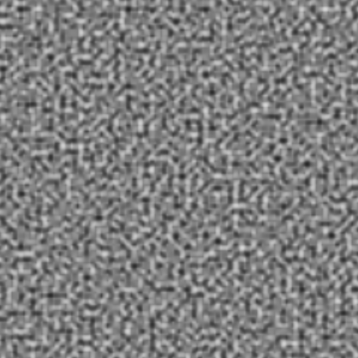
Here's an example of a two dimension slice on a three dimensional implementation with the quintic hermite implementation:


Here's a 2 d example without the quintic smoothing function:


Artifacts more obviously shown.  You can examine the code above for both the two and three dimension forms to see the differences here in implementation.  

Friday, December 5, 2014

Ogre Terrain Height Selection class

 #include <iostream>  

 #include <string>
 #include <sstream>
 #include <vector>
 class Terrainheightselection{
      public:
           Terrainheightselection(Ogre::TerrainGroup* mTerraingroup, Ogre::Vector3 pos, double selsize);
           std::vector<Ogre::Vector3> getSelectionVerts(void);
      private:
           Ogre::TerrainGroup* cmTerraingroup;
           Ogre::Terrain* cterrain;
           float* cheightdata;
           double cselsize;
           Ogre::Vector3 cpos;
           //std::vector<Ogre::Vector3> getSelectionVerts(void);
 };
 Terrainheightselection::Terrainheightselection(Ogre::TerrainGroup* mTerraingroup, Ogre::Vector3 pos, double selsize){
      cmTerraingroup = mTerraingroup;
      cterrain = cmTerraingroup->getTerrain(0,0);
      cheightdata = cterrain->getHeightData();
      cselsize = selsize;
      cpos = pos;
      std::vector<Ogre::Vector3> selverts = getSelectionVerts();
      Ogre::Log* tlog = Ogre::LogManager::getSingleton().getLog("test.log");
      std::ostringstream ss;
      ss<< sizeof(cheightdata);
      tlog->logMessage(ss.str());
      ss.str(std::string());
      ss<< cheightdata[9];
      tlog->logMessage(ss.str());
      Ogre::Real x = cterrain->getSize();
      ss.str(std::string());
      ss<< x;
      tlog->logMessage(ss.str());
      float xd = cterrain->getHeightAtWorldPosition(200,3000,200);
      ss.str(std::string());
      ss<< xd;
      tlog->logMessage(ss.str());
      ss.str(std::string());
      ss<< selverts.size();
      tlog->logMessage(ss.str());
 }
 std::vector<Ogre::Vector3> Terrainheightselection::getSelectionVerts(void){
      Ogre::Real posx, posz;
      Ogre::Real posxmin, posxmax, poszmin, poszmax;
      posx = cpos.x;
      posz = cpos.z;
      posxmin = posx - cselsize;
      posxmax = posx + cselsize;
      poszmin = posz - cselsize;
      poszmax = posz + cselsize;
      std::vector<Ogre::Vector3> veccont;
      for (int i = posxmin; i<posxmax+1; i++){
           for(int j = poszmin; j<poszmax+1; j++){
                double dist = pow(pow(i-posx,2)+pow(j-posz,2),.5);
                if (dist <= cselsize){
 //                    float y = cterrain->getHeightAtWorldPosition(i,3000,j);
                     Ogre::Vector3 retvec;
                     cterrain->getPoint(i,j,&retvec);
                     veccont.push_back(Ogre::Vector3(i,retvec.y,j));
                }
           }
      }
      return veccont;
 }

This class iterates a set of terrain space points using a boundary geometry (square) which the selection tool is confined inside (a circle can be confined in a square whose sides center coincides with the circle's center and whose sides are a distance of 2 * r  where r is the radius of the circle.

I iterate this confining geometry of points to avoid needless computations of points outside such geometry making both point selection faster.  I then point test by checking the the distance such point is less than the falloff radii of the terrain tool (default or user supplied).

Here's a code snippet implementation inside my mouse left button pressed listener

 rlterrVector = Ogre::Vector3(ovec.x,theight,ovec.z);  

           //conver rlterrVector to terrainspace vector
           Ogre::Vector3 rlterrVectorts;
           Ogre::Terrain* cterrain = mTerrainGroup->getTerrain(0,0);
           cterrain->getTerrainPosition(rlterrVector,&rlterrVectorts);
           //terrain space coordinate stored like world space
           crlterrVectorts = Ogre::Vector3(513*rlterrVectorts.x,rlterrVectorts.z,513*rlterrVectorts.y);
           Terrainheightselection* a = new Terrainheightselection(mTerrainGroup, crlterrVectorts,
                                      falloffwidth);
           falloffSelection = a->getSelectionVerts();


In this case I converted the given fixed terrain selection spot, that is, where the user pressed the left mouse button on the given viewport and its corresponding intersection on the given terrain topology, and I converted this from a corresponding world space terrain coordinate selection point (see my blog post on terrain ray query ray testing for tutorial on terrain ray query testing workaround) to terrain space coordinates, and then I pass this to the Terrainheightselection class and grab the selection vertices. You should supply to the this class a position that is in terrain space coordinates but has world space ordering that is, TSvec = (TSvec.x, TSvec.z, TSvec.y)  as is shown above.

I haven't robustly written this by the way for terrain edges (not sure if this will crash if you are for instance adjusting terrain nearest the terrain's edge).

Oblivion

 Between the fascination of an upcoming pandemic ridden college football season, Taylor Swift, and Kim Kardashian, wildfires, crazier weathe...